↗ OpenReview ↗ NeurIPS Homepage ↗ Chat
TL;DR#
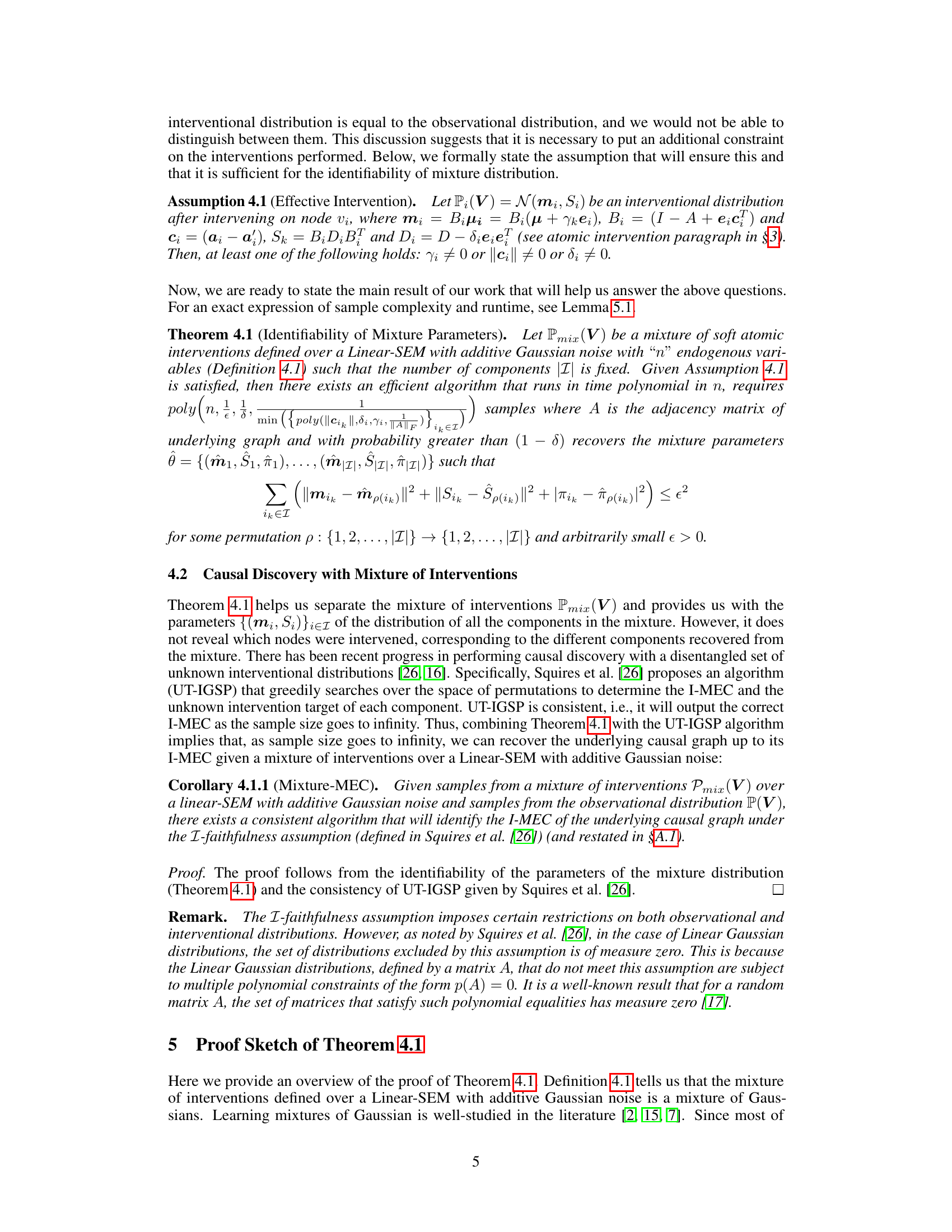
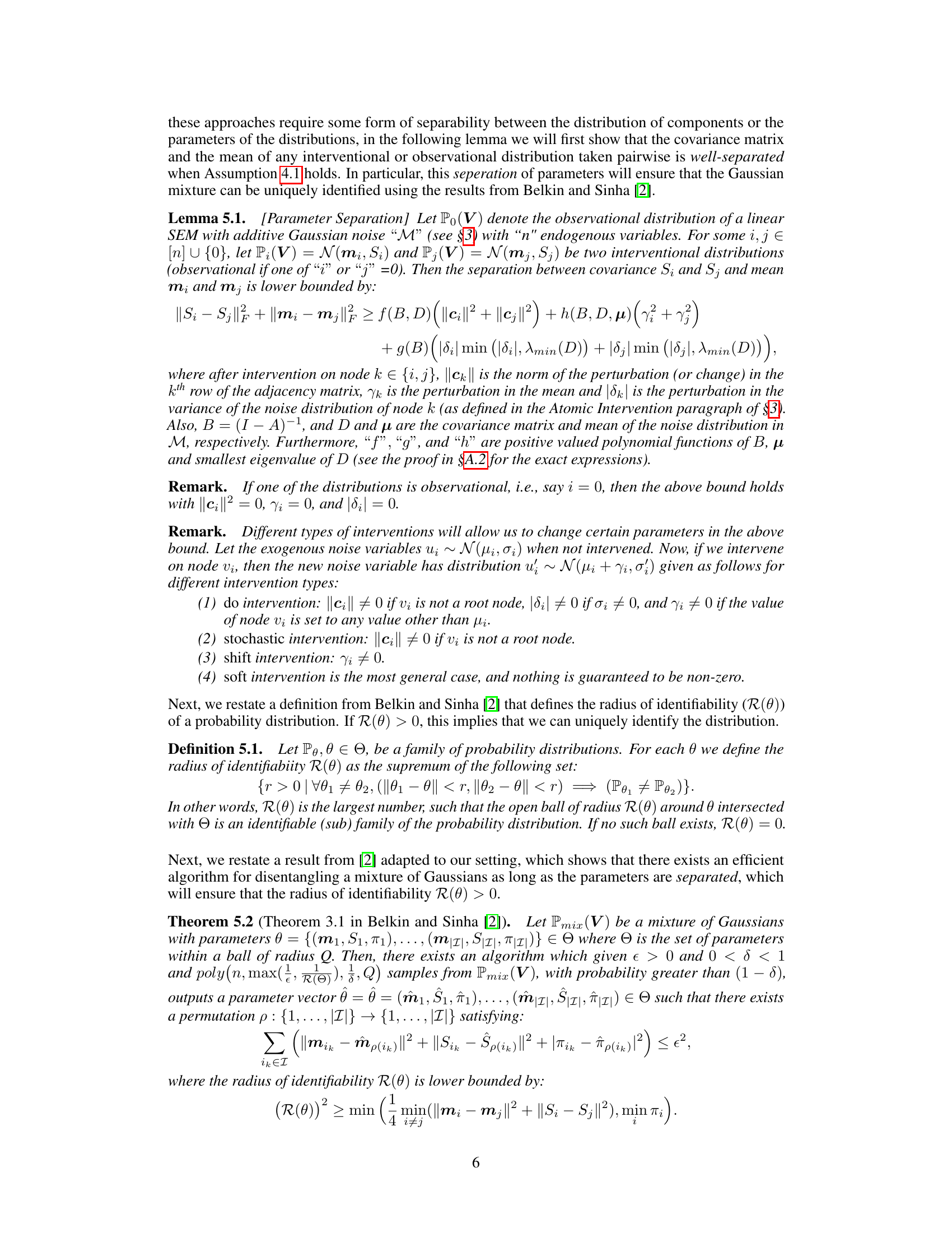
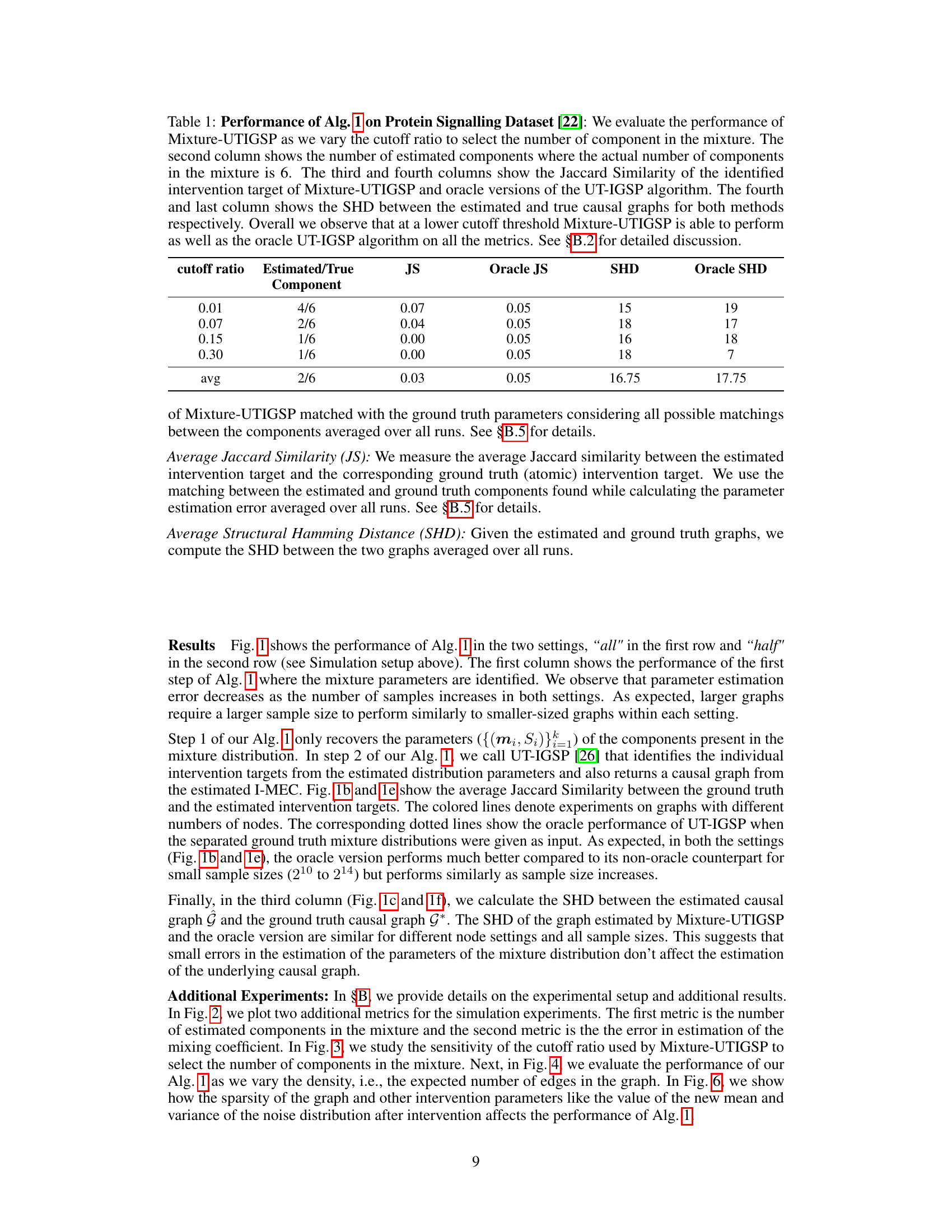
Many real-world applications of causal inference involve interventions, but these interventions often produce noisy data, meaning the data is not solely from the intended intervention but also other sources. This noise makes it challenging to accurately infer causal relationships. Existing methods often struggle with this type of mixed data, leading to unreliable conclusions. This limits their applicability in various fields, such as biology, economics, and social sciences where obtaining perfectly clean interventional data is often difficult or impossible.
This research introduces a new algorithm to address this problem. The algorithm effectively separates noisy interventional data from observational data. This enhanced approach improves the accuracy and reliability of causal inference from datasets containing mixed and imperfect interventional data. The study establishes theoretical guarantees for the method’s accuracy and efficiency, showing its effectiveness in identifying causal relationships even under significant noise. Simulations and real-world experiments verify the algorithm’s performance and capability.
Key Takeaways#
Why does it matter?#
This paper is crucial for researchers in causal inference and machine learning. It addresses a critical limitation in causal discovery by proposing a novel method to handle noisy interventions, which are common in real-world applications. The findings advance causal discovery techniques, enabling more reliable causal relationship identification from complex and imperfect data. This opens doors for more robust and reliable causal analyses across various fields.
Visual Insights#
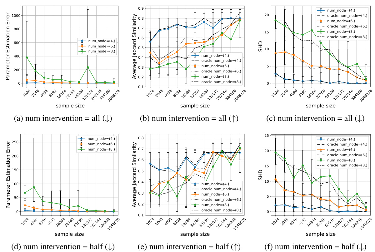
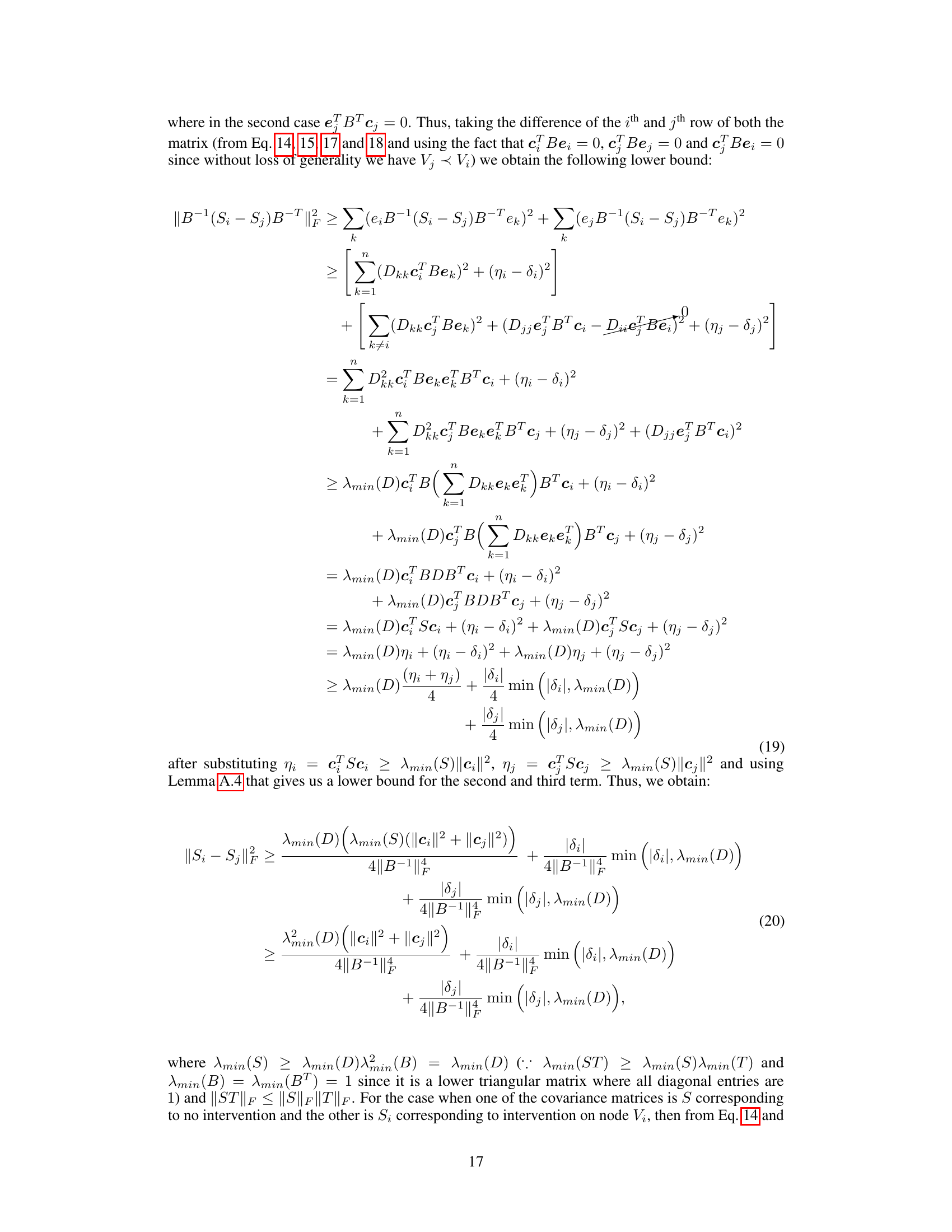
This figure displays the performance of Algorithm 1 across various sample sizes and numbers of nodes. Two scenarios are considered: interventions on all nodes and interventions on half the nodes. The results are shown for three evaluation metrics: Parameter Estimation Error, Average Jaccard Similarity, and Structural Hamming Distance (SHD). The figure demonstrates that increasing sample size generally improves performance, but that larger graphs might need substantially more samples to achieve comparable results to smaller graphs.

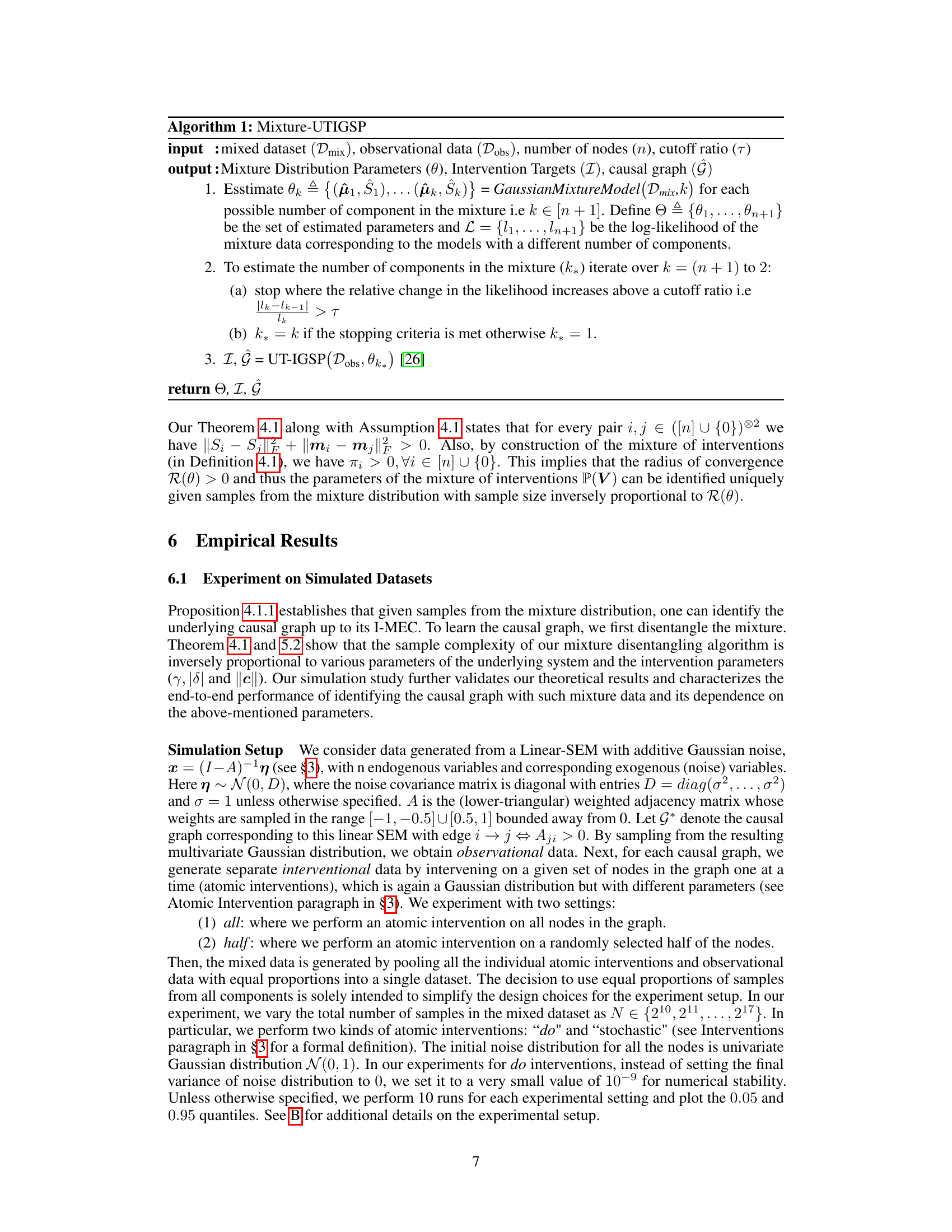
This table presents the results of applying Algorithm 1 (Mixture-UTIGSP) to the protein signaling dataset. It shows how the performance of the algorithm varies with different cutoff ratios used for selecting the number of mixture components. The metrics used for evaluation include the number of estimated components (compared to the actual number, which is 6), Jaccard Similarity (JS) for intervention targets (comparing Mixture-UTIGSP to an oracle UT-IGSP), and Structural Hamming Distance (SHD) between estimated and true causal graphs. The results indicate that Mixture-UTIGSP performs comparably to the oracle method at lower cutoff ratios.
In-depth insights#
Mixed Causal Effects#
The concept of “Mixed Causal Effects” implies scenarios where the impact of a cause on an outcome is not uniform but rather a blend of multiple causal pathways or mechanisms. This complexity arises because multiple causal factors often interact, resulting in effects that are not simply additive. Understanding mixed causal effects is crucial for accurate causal inference, as ignoring the interplay of different mechanisms can lead to biased or incomplete conclusions. For instance, a drug might have a positive effect on a certain subpopulation and a negative effect on another; this requires disentangling the mixed effects to determine the true causal relationship and make well-informed decisions. Identifying and characterizing the different components of mixed effects is a key challenge that requires advanced statistical techniques, potentially involving causal discovery algorithms and modeling approaches that can handle intricate interactions between variables. Addressing confounding variables is essential as they can mask or distort the true nature of mixed causal effects, leading to erroneous causal conclusions. The presence of unobserved or latent confounders further complicates this problem, underscoring the need for robust methods to isolate the impact of each causal pathway. Successfully accounting for these complexities paves the way towards a more nuanced and accurate understanding of causal relationships, enabling more effective interventions in diverse domains.
Intervention Mixtures#
The concept of ‘Intervention Mixtures’ in causal inference research is crucial because it realistically reflects scenarios where interventions are noisy or imprecise. Instead of clean, perfectly targeted interventions, real-world scenarios often involve a blend of intended and unintended effects. This mixing complicates causal discovery, as the observed data is no longer a pure reflection of the intended manipulations. Analyzing these mixtures requires sophisticated methods that can disentangle the different contributions to the observed data, separating the effects of intended interventions from the background noise or unintended side effects. Successfully addressing this challenge is critical for reliable causal inference and the development of effective intervention strategies in fields like genomics, economics and healthcare. Effective techniques for handling intervention mixtures must be robust to uncertainty about the precise nature of the interventions, capable of correctly identifying the causal relationships despite the presence of confounding influences, and computationally efficient to enable analysis of large-scale datasets frequently arising in real-world applications. Ignoring this complexity can lead to misinterpretations of causality and ultimately, ineffective interventions.
Gaussian Mixture#
The concept of a Gaussian Mixture is central to the paper’s approach for disentangling mixed interventional and observational data. The authors leverage the fact that both interventional and observational data, within the linear structural equation model (SEM) framework they employ, result in Gaussian distributions. The challenge becomes how to efficiently and effectively separate (or identify) the individual Gaussian components comprising the mixture, given only samples from the combined distribution. This is a computationally intensive problem, and the authors’ algorithm directly addresses this by showing that under mild conditions, such as the “effective intervention” assumption, the individual Gaussian components (each representing a distinct intervention or observational setting) are identifiable. The efficiency and accuracy of the disentangling algorithm are further demonstrated through simulations. A key insight is that the sample complexity of successfully separating the mixtures is inversely proportional to the magnitude of the changes induced by interventions, implying larger intervention effects improve identifiability. This is critical for applying the disentangled distributions to downstream causal discovery tasks.
Causal Discovery#
Causal discovery, the process of uncovering cause-and-effect relationships from data, is a crucial aspect of this research paper. The paper tackles the challenging problem of disentangling mixed interventional and observational data in causal inference, a situation frequently encountered in real-world applications due to noisy interventions. It focuses on linear structural equation models (SEMs) with Gaussian noise, providing a formal framework for analyzing data where interventions don’t perfectly target intended variables. A key contribution is the development of an efficient algorithm capable of recovering individual interventional distributions from a mixture, even with unknown intervention targets. This involves establishing the identifiability of mixture parameters under certain conditions and demonstrating the algorithm’s effectiveness through simulations. The approach also connects to causal graph identification, showcasing that accurate recovery of interventional distributions can facilitate causal discovery up to the interventional Markov equivalence class, mirroring the results achieved with noise-free interventions. The sample complexity analysis, demonstrating how it scales with problem dimensions and intervention strength, further enhances the work’s significance. Overall, the paper makes notable advances in robust causal inference, offering both theoretical guarantees and practical tools for dealing with the pervasive challenge of noisy interventions in causal discovery.
Algorithm UTIGSP#
The algorithm UTIGSP, likely short for “Uncertain Target Intervention Graph Structure Perturbation”, addresses a crucial challenge in causal discovery: identifying causal relationships from data generated by interventions with unknown targets. This is a significant advancement because in many real-world scenarios, it is difficult to control precisely which variables are intervened upon. UTIGSP cleverly tackles this by exploiting the diversity introduced by noisy interventions and observational data. It leverages the structure of the data to disentangle the various interventional distributions, effectively separating the effects of intended and unintended interventions. Through a series of steps, UTIGSP systematically identifies these separate distributions, revealing much more information about the underlying causal graph. The algorithm likely uses statistical methods like mixture models to separate the overlapping datasets and then applies further steps, potentially using constraint-based or score-based methods, to refine and determine the actual causal structure. The success of UTIGSP hinges on assumptions about the faithfulness of the data and sufficient data sample size to achieve accurate disentanglement. Despite these assumptions, UTIGSP offers a robust approach to causal discovery where precise intervention control is unavailable, opening significant new avenues for research in diverse fields.
More visual insights#
More on figures

This figure displays additional evaluation metrics for the simulation experiments shown in Figure 1. The top row shows results for when all nodes were intervened upon, while the bottom row shows results when only half the nodes were intervened upon. The left column graphs the number of components estimated by the Mixture-UTIGSP algorithm. The right column graphs the error in estimating the mixing weights. Overall, the figure demonstrates that Mixture-UTIGSP accurately estimates the number of components and the mixing weights even with relatively small sample sizes.
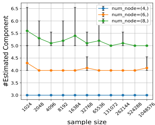
This figure displays the results of two other evaluation metrics, the number of estimated components and the mixing weight estimation error, to complement the results shown in Figure 1. The results are for both the ‘all’ and ‘half’ intervention settings. The number of components estimated by the Mixture-UTIGSP algorithm is shown for different numbers of nodes and sample sizes. The results show that Mixture-UTIGSP accurately estimates the number of components even with a relatively small number of samples. In addition, it is demonstrated that the mixing weight estimation error approaches zero as the sample size increases.
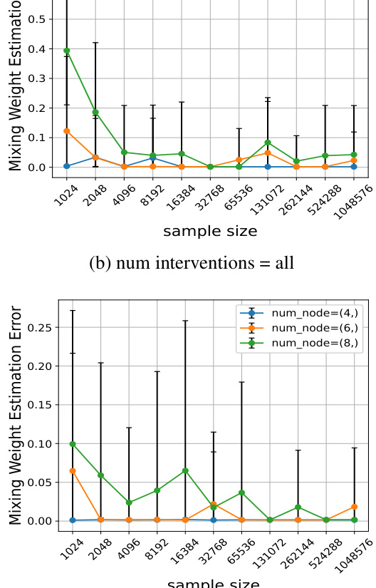
This figure displays two subfigures showing additional evaluation metrics for the simulation experiments in Figure 1. The top subfigure shows the number of estimated components and the mixing weight estimation error for the setting where interventions occur on all nodes. The bottom subfigure shows the same metrics but for the setting where interventions occur on only half of the nodes. In both cases, the results demonstrate that Mixture-UTIGSP accurately estimates the number of components and that the error in estimating mixing weights approaches zero as the sample size increases.

This figure shows how the performance of Algorithm 1 changes when varying the cutoff ratio used for automatic component selection in the mixture model. The experiment considers graphs with 6 nodes and a half-intervention setting. The algorithm selects the number of components using the log-likelihood curve. The figure plots three performance metrics (Parameter Estimation Error, Average Jaccard Similarity, and SHD) against different sample sizes for four cutoff ratios (0.01, 0.15, 0.3, 0.6). The results indicate that for cutoff ratios close to zero, the performance remains consistent, suggesting that the model selection criteria are robust to the choice of cutoff ratio.

This figure shows the performance of Algorithm 1 as the density of the underlying causal graph varies. The experiment uses mixture data with interventions on all nodes plus observational data. Three evaluation metrics are plotted: Parameter Estimation Error, Average Jaccard Similarity, and Structural Hamming Distance (SHD). As graph density increases, more samples are needed to achieve similar performance because the sample complexity is proportional to the norm of the adjacency matrix, which increases with density.
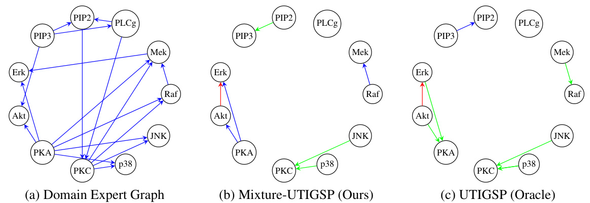
This figure compares the ground truth causal graph from domain experts with the causal graphs estimated by the Mixture-UTIGSP algorithm (proposed in the paper) and the UTIGSP algorithm (from prior work) using the Protein Signaling dataset. The comparison highlights the accuracy of the Mixture-UTIGSP algorithm in recovering the true causal relationships, showing it performs comparably to the UTIGSP algorithm which is given the advantage of already having disentangled the mixture data.

This figure empirically validates Theorem 4.1 by showing how changing the mean and variance of the noise distribution in interventions affects the performance of the proposed algorithm. It demonstrates that larger changes in these parameters lead to better performance (lower estimation error, higher Jaccard similarity, lower Structural Hamming Distance) across different sample sizes.

This figure empirically validates Theorem 4.1 of the paper, which states that the sample complexity for recovering the parameters of the mixture is inversely proportional to the magnitude of changes induced by an intervention. Three subplots show how the Parameter Estimation Error, Average Jaccard Similarity, and Structural Hamming Distance (SHD) change as sample size increases. Each subplot further explores how these metrics change when either the mean (yi) or variance (|δi|) of the noise distribution is varied after an intervention. The results show that larger changes in the mean and variance lead to improved performance (lower error and higher similarity/accuracy) as expected from the theoretical analysis. Specifically, as the magnitude of intervention change increases, the recovery is more robust, even for smaller sample sizes.
Full paper#
