TL;DR#
Few-shot node classification (FSNC) is a challenging task where Graph Neural Networks (GNNs) struggle due to their tendency to overfit limited labeled data and underperform on unseen classes. Existing approaches, such as Sharpness-Aware Minimization (SAM), aim to improve generalization but often come at a high computational cost. This limits their practical applicability, especially in resource-constrained settings.
To address these challenges, this paper proposes Fast Graph Sharpness-Aware Minimization (FGSAM). FGSAM leverages the strengths of both GNNs and Multi-Layer Perceptrons (MLPs) to find a balance between performance and efficiency. It reuses gradients from a perturbation step to incorporate graph topology information into the minimization process without adding significant computational cost, leading to substantial efficiency gains. Further enhancements are made in FGSAM+, executing exact perturbations periodically to further optimize training.
Key Takeaways#
Why does it matter?#
This paper is important because it addresses the challenge of improving the generalization ability of Graph Neural Networks (GNNs) in few-shot node classification (FSNC) tasks. It introduces a novel and efficient algorithm, significantly advancing the state-of-the-art in GNN training for FSNC and opening new avenues for research in efficient model generalization and graph learning.
Visual Insights#

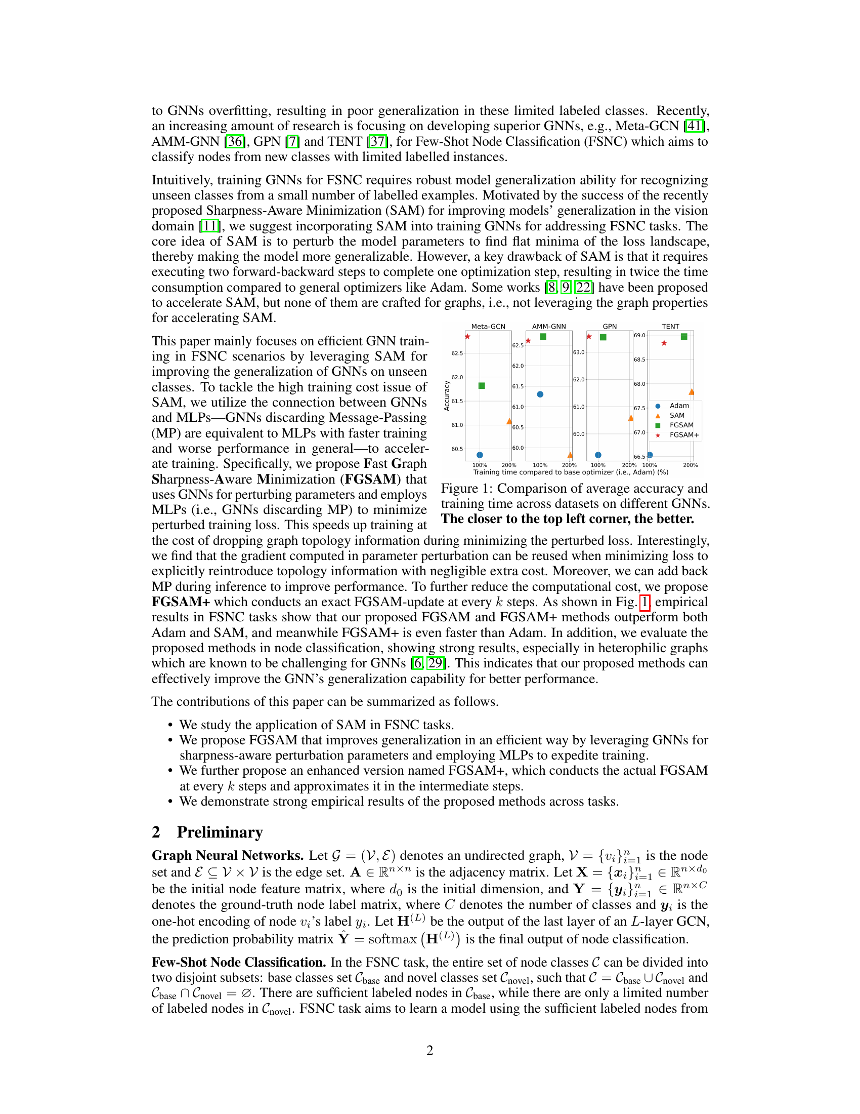
🔼 This figure compares the performance of several GNNs (Meta-GCN, AMM-GNN, GPN, TENT) optimized using different methods (Adam, SAM, FGSAM, FGSAM+). It visualizes the trade-off between accuracy and training time. Each point represents a GNN trained with a specific optimization algorithm on a specific dataset. The x-axis shows the training time relative to the Adam optimizer (100% representing the training time of Adam), and the y-axis represents the average accuracy achieved on various datasets. The top left corner represents the ideal scenario—high accuracy and low training time. The figure suggests that FGSAM+ achieves a good balance between these two aspects, outperforming other methods in many cases.
read the caption
Figure 1: Comparison of average accuracy and training time across datasets on different GNNs. The closer to the top left corner, the better.

🔼 This table presents the time it took to train different models for 200 episodes using two different methods: one with message passing (GNN) and one without (PeerMLP). The results are broken down by dataset (CoraFull, DBLP, ogbn-A) and model type (GNN, PeerMLP). It shows that PeerMLP is significantly faster than GNN but might not generalize well.
read the caption
Table 1: Time consumption of 200 episodes training (sec.) of baseline w/ and w/o MP (only consider feed-forward and -backward).
In-depth insights#
FSNC via SAM#
The application of Sharpness-Aware Minimization (SAM) to Few-Shot Node Classification (FSNC) presents a compelling approach to enhance model generalization. SAM’s core strength lies in finding flat minima in the loss landscape, leading to improved robustness against overfitting, a critical concern in FSNC due to limited labeled data for novel classes. However, the standard SAM algorithm’s computational overhead, stemming from its two forward-backward steps per iteration, poses a significant challenge. Therefore, integrating SAM efficiently into GNN training is crucial. The research explores ways to leverage the relationship between GNNs and MLPs to accelerate SAM’s training while retaining the benefits of GNNs’ superior performance on graph data. The resulting method aims for an optimal trade-off between computational efficiency and the generalization power offered by SAM, ultimately striving for improved FSNC accuracy and faster training times.
FGSAM Algorithmic#
A hypothetical “FGSAM Algorithmic” section would delve into the detailed steps and mathematical formulations of the proposed Fast Graph Sharpness-Aware Minimization algorithm. It would likely begin by explaining the rationale behind using GNNs for parameter perturbation and MLPs for loss minimization, highlighting the efficiency gains compared to standard SAM. A key aspect would be a precise description of how graph topology is reintroduced into the minimization process, potentially using a technique to reuse gradients from the perturbation phase. The section would also present the algorithmic steps, likely in pseudocode or a flow chart, clearly outlining the calculations involved in each iteration. Finally, the discussion might cover algorithmic variations like FGSAM+, which introduces periodic exact perturbations, to further optimize training efficiency, and the resulting computational tradeoffs involved. The core focus of such a section would be clarity, precision, and a demonstrable connection between the algorithm’s design and its intended performance benefits.
GNN-MLP Synergy#
The concept of “GNN-MLP Synergy” in the context of few-shot node classification suggests a powerful combination of Graph Neural Networks (GNNs) and Multi-Layer Perceptrons (MLPs). GNNs excel at capturing complex graph structural information, crucial for node classification, but can be computationally expensive and prone to overfitting. MLPs, on the other hand, offer faster training and better generalization, but lack the ability to directly model graph structures. A synergistic approach would leverage GNNs for the initial parameter perturbation phase of sharpness-aware minimization (SAM), effectively using their power to find a flat minimum in the loss landscape. Then, by switching to MLPs for loss minimization, one can combine the strengths of both models: GNNs’ structural awareness for better generalization and MLPs’ computational efficiency for faster training. The key is finding a way to reintroduce the graph topology information back into the loss minimization stage, preferably with minimal extra computational overhead, to avoid the performance loss of using MLPs solely. This fusion of GNNs and MLPs, ideally with a clever strategy to retain the graph information, is what makes this ‘synergy’ promising for few-shot node classification.
Efficiency & Speed#
The research paper emphasizes achieving efficiency and speed in its proposed method, particularly within the context of few-shot node classification. A key contribution is the Fast Graph Sharpness-Aware Minimization (FGSAM) algorithm, which aims to overcome the computational limitations of traditional SAM methods by strategically integrating the rapid training of Multi-Layer Perceptrons (MLPs) with the superior performance of Graph Neural Networks (GNNs). FGSAM reuses the gradient from a parameter perturbation phase, reducing computational costs significantly. Further enhancing efficiency, FGSAM+ periodically executes exact perturbations, allowing for faster training while maintaining accuracy. Empirical results demonstrate that these methods outperform standard SAM with reduced training times, making them particularly suitable for resource-constrained settings. The focus on efficiency is a significant strength, making the method more practical for real-world applications.
Future Works#
Future research directions stemming from this paper could explore extending FGSAM to more complex graph structures beyond those tested, and investigating its performance on larger-scale datasets. A key area is developing theoretical guarantees for FGSAM’s efficiency and generalization, potentially analyzing its convergence properties under various graph topologies and data distributions. Another promising avenue is combining FGSAM with other techniques for enhancing few-shot node classification, such as meta-learning or data augmentation methods. Finally, the application of FGSAM to other graph learning tasks beyond node classification warrants exploration, such as graph clustering and link prediction, assessing its potential advantages in these diverse contexts. Investigating the robustness of FGSAM to noisy or incomplete graph data is also important for practical applications.
More visual insights#
More on figures

🔼 This figure visualizes the loss landscape and loss curve for GNNs, MLPs, and PeerMLPs across different tasks (node classification and few-shot node classification) and optimizers. The loss landscapes illustrate the difference in the complexity of the loss function for each setting. The loss curves show the test loss over the training process, highlighting the faster convergence and improved generalization of PeerMLP and FGSAM compared to GNNs with standard optimizers.
read the caption
Figure 2: (a): Loss landscape visualization of GNN across tasks and optimizers. (b): Loss of GNN, MLP and its PeerMLP on the test set over the training process. In these experiments, MLP and PeerMLP share the same weight space as GNN but are trained without message-passing.
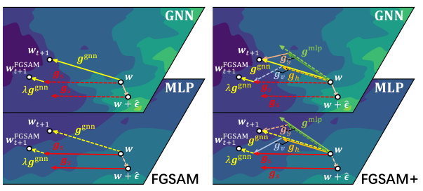
🔼 This figure visualizes the framework of FGSAM and FGSAM+ and shows the difference of gradients across the training process for both algorithms. The left panel (a) shows that the solid line represents gradients calculated on the corresponding model. The dashed line represents the gradient computed on the opposite model, while the right panel (b) shows how the differences in gradients change much slower than gs and gh. Therefore, gv and gg can be reused in intermediate steps to save computational cost.
read the caption
Figure 3: Left (a): The solid line indicates that the gradient is computed on the corresponding model, while the dashed line indicates the opposite. Right (b): The difference of gradients (i.e., ||gt+1−gt||2). It can be seen that gv and gg change much slower than gs and gh across the training process, thus can be reused in the intermediate steps.

🔼 This figure visualizes the framework of FGSAM and FGSAM+ and shows the difference of gradients across the training process for different components. The left panel (a) shows a schematic of the two algorithms, with solid lines representing gradients computed on the corresponding model and dashed lines representing the opposite. The right panel (b) shows that the differences in gradients (gv and gg) change much slower compared to others (gs and gh), indicating that they can be reused in intermediate steps for computational efficiency.
read the caption
Figure 3: Left (a): The solid line indicates that the gradient is computed on the corresponding model, while the dashed line indicates the opposite. Right (b): The difference of gradients (i.e., ||gt+1-gt||2). It can be seen that gv and gg change much slower than gs and gh across the training process, thus can be reused in the intermediate steps.

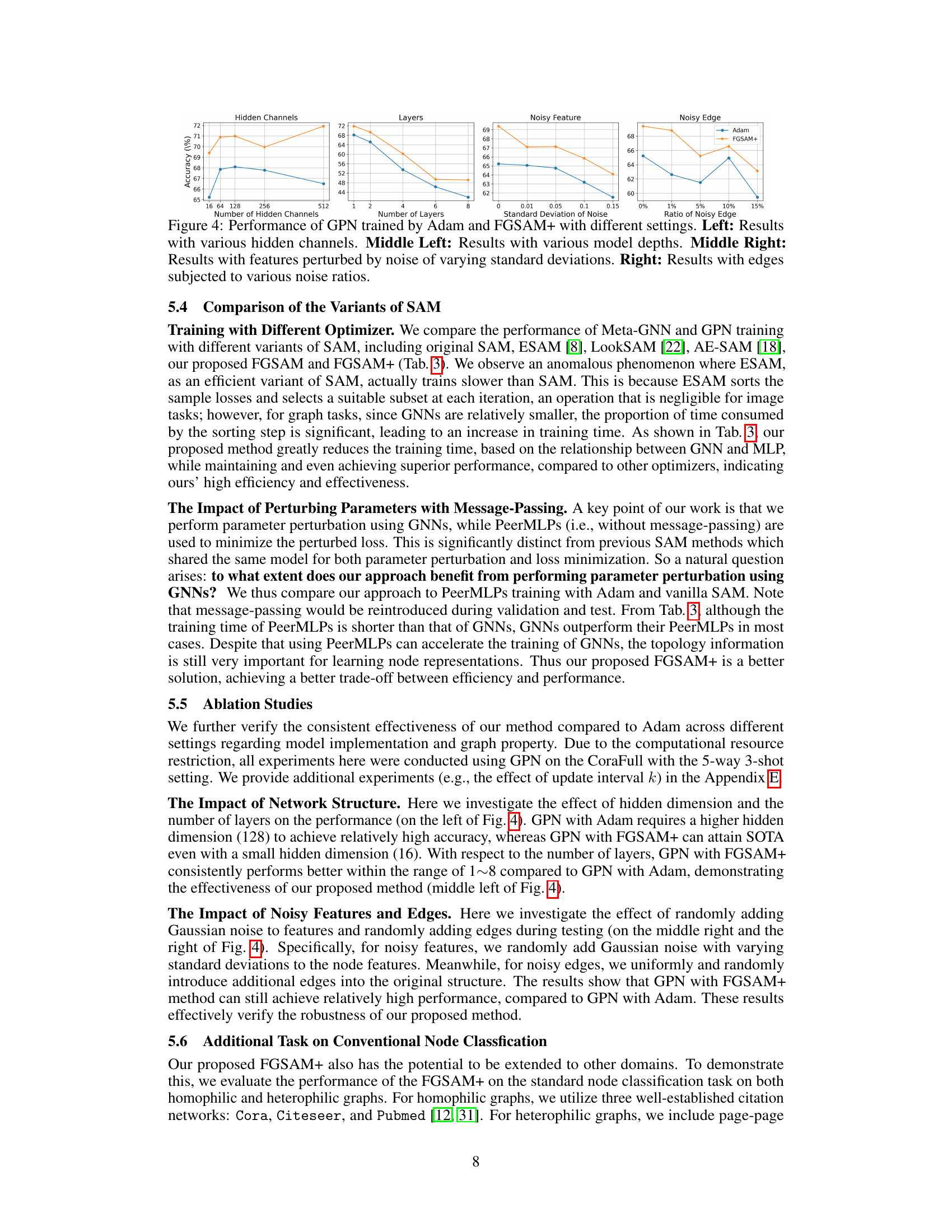
🔼 This figure presents the results of experiments conducted to evaluate the performance of Graph Prototypical Networks (GPN) trained using two different optimizers: Adam and FGSAM+. The experiments were designed to investigate the impact of various hyperparameters on the model’s performance. Four different aspects were examined: 1. Number of Hidden Channels: The leftmost plot shows how accuracy changes with varying numbers of hidden channels in the GPN architecture. 2. Number of Layers: The next plot illustrates the effect of the number of layers in the GPN model on accuracy. 3. Noisy Features: The third plot explores the impact of adding Gaussian noise to the input features (with varying standard deviations) on the model’s accuracy. 4. Noisy Edges: The final plot examines the influence of randomly adding edges to the graph (with various ratios of noisy edges to the original number of edges) on the GPN’s accuracy. Each plot compares the accuracy achieved using Adam against the accuracy achieved using FGSAM+, allowing for a direct comparison of their performance under different conditions.
read the caption
Figure 4: Performance of GPN trained by Adam and FGSAM+ with different settings. Left: Results with various hidden channels. Middle Left: Results with various model depths. Middle Right: Results with features perturbed by noise of varying standard deviations. Right: Results with edges subjected to various noise ratios.
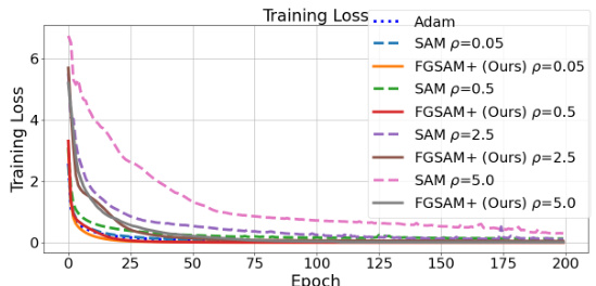
🔼 The figure shows training loss curves for different values of hyperparameter p (radius of the lp ball) across various optimizers: Adam, SAM, and FGSAM+. It illustrates how the training loss converges differently depending on the optimizer and the value of p. Specifically, it demonstrates that SAM struggles to converge with higher p values, while FGSAM+ consistently achieves convergence. This highlights FGSAM+’s ability to mitigate the issues associated with imbalanced adversarial games in SAM-like methods.
read the caption
Figure 5: Training loss curves related to different p across optimizers.

🔼 This figure shows two plots. Plot (a) visualizes the framework of FGSAM and FGSAM+. The solid lines represent the gradient being computed on the corresponding model (GNN or MLP), while the dashed lines indicate the opposite. Plot (b) displays curves showing the difference in gradients (||gt+1-gt||2) during training. The figure demonstrates that the gradient variation for gv and gg is significantly slower than that for gs and gh, supporting the claim that gv and gg can be reused to enhance computational efficiency in intermediate training steps.
read the caption
Figure 3: Left (a): The solid line indicates that the gradient is computed on the corresponding model, while the dashed line indicates the opposite. Right (b): The difference of gradients (i.e., ||gt+1-gt||2). It can be seen that gv and gg change much slower than gs and gh across the training process, thus can be reused in the intermediate steps.
More on tables

🔼 This table presents the accuracy and training time of several state-of-the-art (SOTA) models for few-shot node classification (FSNC) using different optimizers: Adam, SAM, FGSAM, and FGSAM+. The results are shown for different dataset settings (5-way 3-shot, 5-way 5-shot, 10-way 3-shot, and 10-way 5-shot) across three datasets: CoraFull, DBLP, and ogbn-arXiv. The table highlights the best performing model for each setting using bold text and the second-best performing model using underlined text. It also provides the training time for 200 episodes, focusing solely on the feedforward and backpropagation steps.
read the caption
Table 2: Accuracy and Time consumption on the baseline with different optimizer. The best and the runner-up are denoted as boldface and underlined, respectively. '5N3K' denotes 5-way 3-shot setting. Time consumption of 200 episodes of training (sec., only consider forward-backward) is also shown.

🔼 This table presents the accuracy and training time of several state-of-the-art models using different optimizers (Adam, SAM, FGSAM, and FGSAM+) under various few-shot learning settings (5-way 3-shot, 5-way 5-shot, 10-way 3-shot, and 10-way 5-shot). It compares the performance of these optimizers across three different datasets: CoraFull, DBLP, and ogbn-arXiv. The time reported is for 200 training epochs and only includes the forward and backward passes. The best and second-best accuracies are highlighted in bold and underlined, respectively.
read the caption
Table 2: Accuracy and Time consumption on the baseline with different optimizer. The best and the runner-up are denoted as boldface and underlined, respectively. '5N3K' denotes 5-way 3-shot setting. Time consumption of 200 episodes of training (sec., only consider forward-backward) is also shown.

🔼 This table presents the accuracy and training time of several baseline models (Meta-GCN, AMM-GNN, GPN, TENT) using different optimizers (Adam, SAM, FGSAM, FGSAM+). The results are shown for various few-shot learning settings (5-way 3-shot, 5-way 5-shot, 10-way 3-shot, 10-way 5-shot) across three datasets (CoraFull, DBLP, ogbn-arXiv). The table highlights the best-performing models and optimizers in terms of accuracy and training time efficiency.
read the caption
Table 2: Accuracy and Time consumption on the baseline with different optimizer. The best and the runner-up are denoted as boldface and underlined, respectively. '5N3K' denotes 5-way 3-shot setting. Time consumption of 200 episodes of training (sec., only consider forward-backward) is also shown.

🔼 This table presents the statistics of three benchmark node classification datasets used in the paper’s experiments. For each dataset (CoraFull, DBLP, and ogbn-arXiv), it shows the number of nodes, edges, features, and classes. It also provides the class split used for training, validation, and testing, showing the percentage of nodes allocated to each set.
read the caption
Table 5: Statistics of evaluation datasets

🔼 This table presents the accuracy and training time for different optimizers (Adam, SAM, FGSAM, FGSAM+) applied to various GNN models (Meta-GCN, AMM-GNN, GPN, TENT) on three datasets (CoraFull, DBLP, ogbn-arXiv) with 5-way 3-shot and 5-way 5-shot settings. The best and second-best results are highlighted.
read the caption
Table 2: Accuracy and Time consumption on the baseline with different optimizer. The best and the runner-up are denoted as boldface and underlined, respectively. '5N3K' denotes 5-way 3-shot setting. Time consumption of 200 episodes of training (sec., only consider feed-forward and -backward) is also shown.
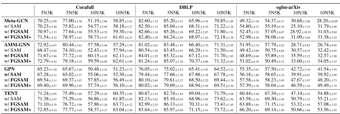
🔼 This table presents the accuracy and training time of several state-of-the-art models (Meta-GCN, AMM-GNN, GPN, TENT) using different optimizers (Adam, SAM, FGSAM, FGSAM+) in the 5-way 3-shot setting. The results are presented for three different datasets (CoraFull, DBLP, ogbn-arXiv). The table shows that FGSAM and FGSAM+ generally achieve higher accuracy compared to Adam and SAM, while FGSAM+ achieves faster training speed than Adam in most cases.
read the caption
Table 2: Accuracy and Time consumption on the baseline with different optimizer. The best and the runner-up are denoted as boldface and underlined, respectively. '5N3K' denotes 5-way 3-shot setting. Time consumption of 200 episodes of training (sec., only consider feed-forward and -backward) is also shown.

🔼 This table presents the accuracy and training time of various models (Meta-GCN, AMM-GNN, GPN, TENT) using different optimizers (Adam, SAM, FGSAM, FGSAM+) on three datasets (CoraFull, DBLP, ogbn-arXiv) under different few-shot learning settings (5N3K, 5N5K, 10N3K, 10N5K). The results show that FGSAM and FGSAM+ generally outperform Adam and SAM, particularly in terms of training time.
read the caption
Table 2: Accuracy and Time consumption on the baseline with different optimizer. The best and the runner-up are denoted as boldface and underlined, respectively. ‘5N3K’ denotes 5-way 3-shot setting. Time consumption of 200 episodes of training (sec., only consider feed-forward and -backward) is also shown.

🔼 This table presents the accuracy and training time of several state-of-the-art models for few-shot node classification on three datasets (CoraFull, DBLP, ogbn-arXiv) under different optimization methods (Adam, SAM, FGSAM, FGSAM+). The results are shown for various few-shot settings (5-way 3-shot, 5-way 5-shot, 10-way 3-shot, 10-way 5-shot). The training times are also provided for 200 episodes of training, focusing only on the forward and backward passes, showcasing the computational efficiency of the proposed methods.
read the caption
Table 2: Accuracy and Time consumption on the baseline with different optimizer. The best and the runner-up are denoted as boldface and underlined, respectively. '5N3K' denotes 5-way 3-shot setting. Time consumption of 200 episodes of training (sec., only consider feed-forward and -backward) is also shown.

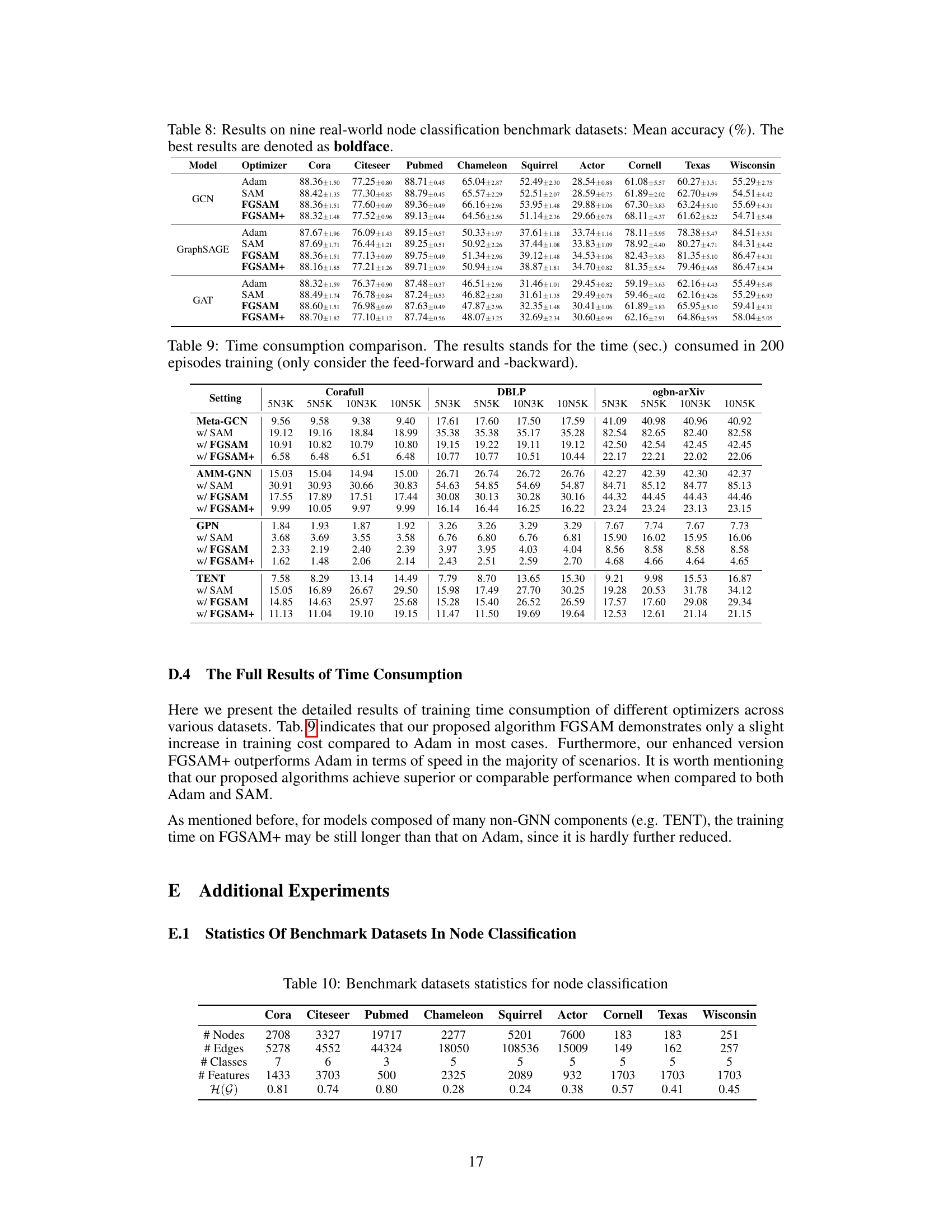
🔼 This table presents the statistics of nine real-world benchmark datasets used for node classification in the paper. For each dataset, it provides the number of nodes, edges, classes, features, and the homophily score H(G). The homophily score is a measure of how likely nodes of the same class are to be connected. Datasets include Cora, Citeseer, Pubmed, Chameleon, Squirrel, Actor, Cornell, Texas, and Wisconsin.
read the caption
Table 10: Benchmark datasets statistics for node classification

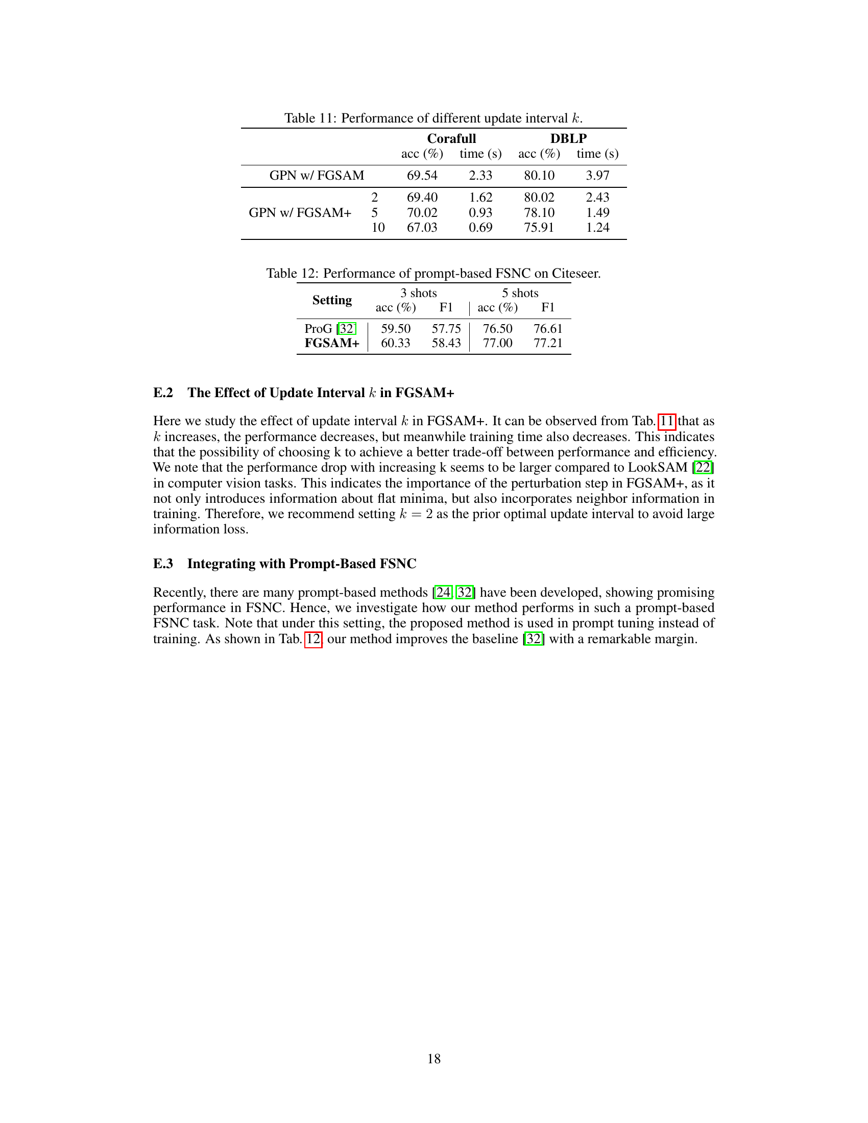
🔼 This table presents the performance of GPN with FGSAM+ using different update intervals (k). It shows that as k increases, the accuracy decreases, but the training time also decreases, indicating a trade-off between accuracy and training efficiency. The results are shown for CoraFull and DBLP datasets, showcasing the impact of the update interval on both accuracy and training time.
read the caption
Table 11: Performance of different update interval k.

🔼 This table presents the results of prompt-based few-shot node classification (FSNC) on the Citeseer dataset. It compares the performance of the baseline method, ProG [32], against the proposed FGSAM+ method. The comparison is shown for both 3-shot and 5-shot settings, with accuracy (acc) and F1-score (F1) reported for each.
read the caption
Table 12: Performance of prompt-based FSNC on Citeseer.
Full paper#

