TL;DR#
High-dimensional data, common in fields like genomics and single-cell biology, poses a challenge for machine learning models. Existing methods, like PCA, struggle to capture human-understandable concepts, while deep learning models are often ‘black boxes’, lacking interpretability. Furthermore, existing methods fail to effectively model data spread across multiple subspaces, limiting their ability to tease apart different underlying processes.
The paper introduces Supervised Independent Subspace Principal Component Analysis (sisPCA), a new method designed to overcome these limitations. sisPCA uses supervision (e.g., known labels) to guide the decomposition of data into multiple independent subspaces that are clearly interpretable. Using various biological datasets, the authors demonstrate sisPCA’s ability to accurately identify and separate data structures associated with biological processes, revealing insights otherwise missed by traditional methods.
Key Takeaways#
Why does it matter?#
This paper is crucial for researchers working with high-dimensional data, particularly in biology and medicine. It provides a novel method, sisPCA, for interpretable data analysis, addressing the limitations of existing techniques. sisPCA’s ability to disentangle multiple factors and integrate supervision opens new avenues for understanding complex biological systems and can accelerate progress in various fields, such as genomics and single-cell analysis.
Visual Insights#

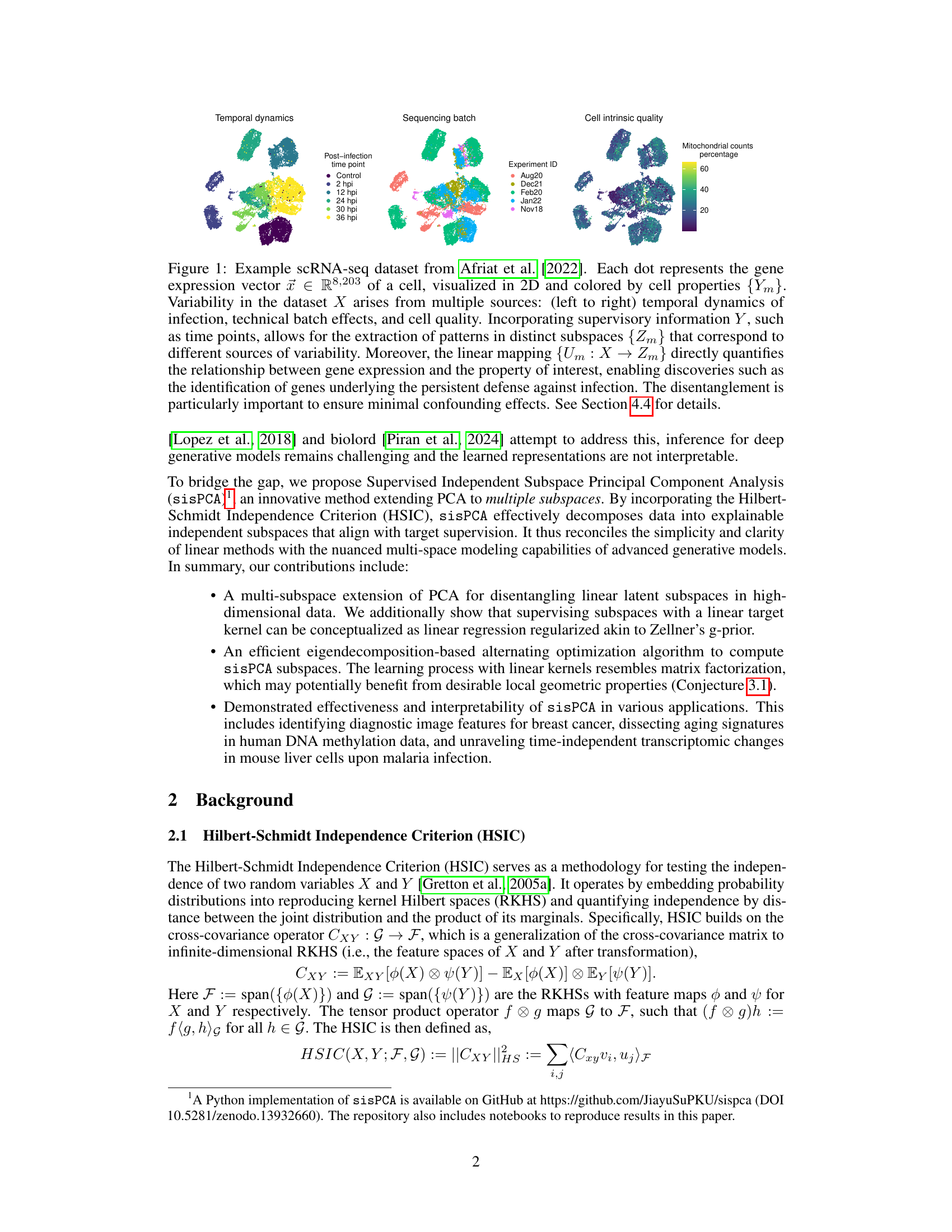
🔼 This figure shows an example of scRNA-seq data visualized in 2D. Each point represents a cell’s gene expression profile. The data’s variability comes from various sources, including temporal dynamics of infection, technical batch effects, and cell quality. The figure demonstrates how supervised subspace learning can separate these sources of variability into distinct subspaces.
read the caption
Figure 1: Example scRNA-seq dataset from Afriat et al. [2022]. Each dot represents the gene expression vector F∈ R8,203 of a cell, visualized in 2D and colored by cell properties {Ym}. Variability in the dataset X arises from multiple sources: (left to right) temporal dynamics of infection, technical batch effects, and cell quality. Incorporating supervisory information Y, such as time points, allows for the extraction of patterns in distinct subspaces {Zm} that correspond to different sources of variability. Moreover, the linear mapping {Um: X → Zm} directly quantifies the relationship between gene expression and the property of interest, enabling discoveries such as the identification of genes underlying the persistent defense against infection. The disentanglement is particularly important to ensure minimal confounding effects. See Section 4.4 for details.

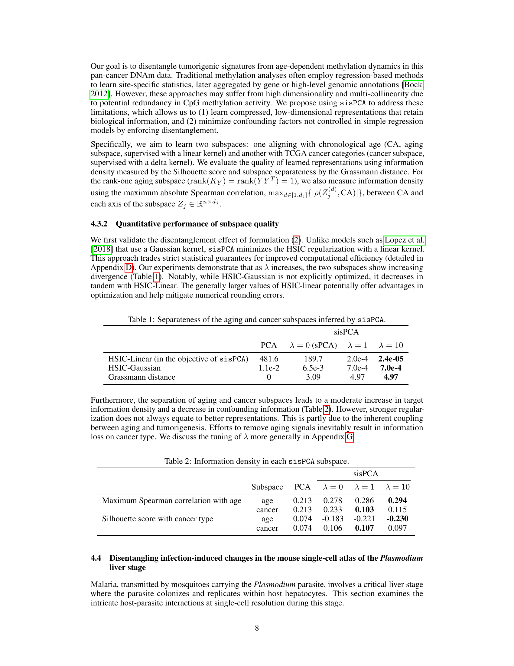
🔼 This table presents the results of applying sisPCA with different values of the regularization parameter λ to separate aging and cancer subspaces. It shows the HSIC values (both linear and Gaussian kernels) and the Grassmann distance between the subspaces. The HSIC measures the dependence between the subspaces, while the Grassmann distance quantifies their separability. The results demonstrate that increasing λ leads to a greater separation of the aging and cancer subspaces, suggesting that it effectively controls for confounding factors during subspace disentanglement. λ = 0 represents the supervised PCA (sPCA) baseline.
read the caption
Table 1: Separateness of the aging and cancer subspaces inferred by sisPCA.
In-depth insights#
sisPCA: A New PCA#
The heading “sisPCA: A New PCA” suggests a novel extension of Principal Component Analysis (PCA). This implies sisPCA retains PCA’s core functionality of dimensionality reduction but introduces significant enhancements. The “supervised independent subspace” aspect points towards an algorithm that leverages labeled data to decompose high-dimensional data into multiple independent subspaces. This is a substantial departure from traditional PCA, which is unsupervised, and likely addresses a key limitation of PCA: its inability to directly incorporate prior knowledge or supervision. The independence of the subspaces suggests that sisPCA aims to disentangle underlying factors that may be confounded in the original data, allowing for a more interpretable representation. The novelty implied by the term “new PCA” suggests that sisPCA may offer improvements in either computational efficiency, accuracy, or interpretability compared to existing methods, potentially achieving superior performance in specific application domains requiring structured data decompositions.
Multi-Subspace Learning#
Multi-subspace learning tackles the challenge of representing high-dimensional data by decomposing it into multiple, independent subspaces. This approach is particularly valuable when the data exhibits complex, interwoven patterns stemming from different underlying factors or sources. Unlike traditional methods like PCA, which find a single optimal subspace, multi-subspace learning aims to identify several subspaces that capture distinct aspects of the data. This disentanglement of factors improves interpretability, allowing researchers to understand the individual contributions of different sources of variation, rather than a single, aggregate representation. The independence between subspaces is crucial, as it prevents the confounding of distinct data structures and enables a more accurate and nuanced interpretation of the data. This strategy is especially relevant in domains such as biology or medicine where the high dimensionality of the data makes it difficult to uncover underlying patterns and relationships. Supervised versions of multi-subspace learning further enhance the process by incorporating external information or labels to guide the subspace discovery, thereby linking the identified structures to specific variables or features of interest. In essence, multi-subspace learning offers a powerful tool for exploring and understanding complex data by revealing its underlying latent structure in a more insightful and interpretable manner.
HSIC in sisPCA#
The core of sisPCA lies in its innovative integration of the Hilbert-Schmidt Independence Criterion (HSIC). HSIC elegantly quantifies the dependence between two random variables, mapped into Reproducing Kernel Hilbert Spaces (RKHS). In sisPCA, HSIC plays a dual role: first, maximizing HSIC between each subspace and its corresponding supervisory variable ensures that the learned subspace captures the relevant information related to the target. Second, minimizing HSIC between different subspaces promotes independence and disentanglement, preventing confounding effects and enabling a more interpretable representation of the data. This clever use of HSIC is what sets sisPCA apart from traditional PCA methods and allows it to effectively model high-dimensional data with multiple, independent latent structures, thereby resolving the challenge of interpretability in many multi-subspace learning scenarios. The careful balancing of these HSIC terms, controlled by the regularization parameter λ, is crucial for achieving optimal subspace separation and interpretability.
sisPCA Applications#
The ‘sisPCA Applications’ section showcases the model’s versatility across diverse biological datasets. High-dimensional data, such as breast cancer images, aging-related DNA methylation patterns, and malaria infection single-cell RNA sequencing, are effectively analyzed. SisPCA’s ability to disentangle subspaces reveals distinct functional pathways in malaria colonization, highlighting the importance of interpretable representations. Comparison with existing methods like PCA and sPCA demonstrates sisPCA’s superior performance in separating independent data sources and improving diagnostic prediction accuracy. The use of simulated data validates sisPCA’s ability to recover both supervised and unsupervised subspaces, demonstrating its robustness and effectiveness. The findings underscore sisPCA’s potential as a powerful tool for uncovering hidden biological insights within complex, high-dimensional data, leading to more accurate interpretations and improved decision-making.
sisPCA Limitations#
sisPCA, while offering a novel approach to multi-subspace learning, is not without limitations. Linearity constraints restrict its ability to capture complex non-linear relationships within data. The reliance on linear kernels for HSIC regularization, while computationally efficient, may not fully guarantee statistical independence between subspaces. Furthermore, the method’s dependence on external supervision for subspace identification could lead to identifiability issues if supervision is weak or subspaces are similar. The success of sisPCA is also influenced by the choice of hyperparameters, particularly the regularization parameter (λ), which requires careful tuning to balance subspace independence and dependence on target variables. Finally, while the method is designed for interpretability, the performance and meaning of results might vary with dataset characteristics, highlighting the need for robust validation across diverse applications.
More visual insights#
More on figures

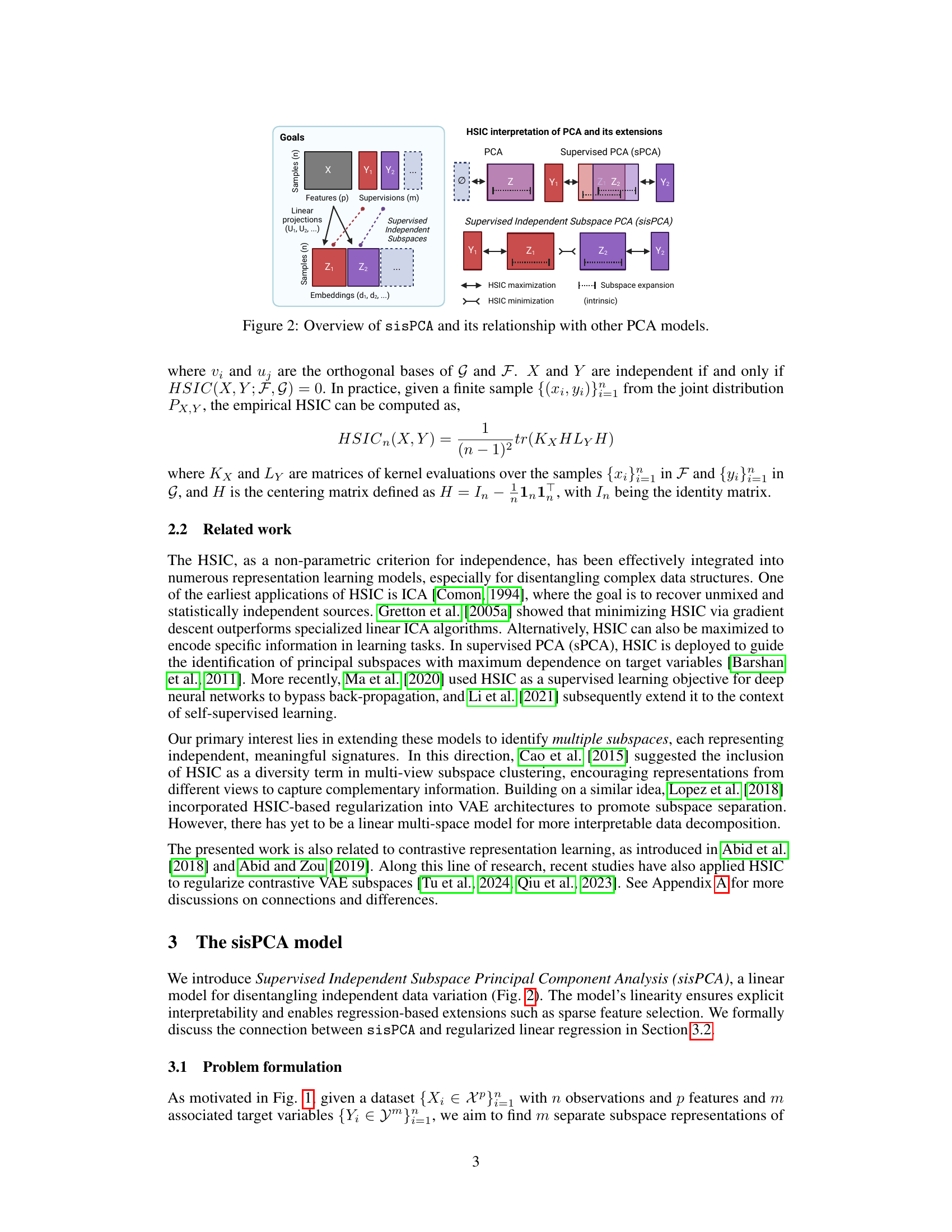
🔼 This figure illustrates the relationship between sisPCA and other principal component analysis (PCA) methods. It shows how sisPCA extends PCA by incorporating supervision and simultaneously ensuring subspace disentanglement, unlike traditional PCA or supervised PCA which only model single subspace or supervised single subspace respectively. The figure highlights the goals of each method (e.g., finding orthogonal bases and maximizing dependence with target variables while minimizing overlap between subspaces). The HSIC (Hilbert-Schmidt Independence Criterion) is used as a measure of dependence between the subspaces and the supervision variables. SisPCA uses HSIC maximization to learn subspace projections that maximize dependence with target variables and HSIC minimization to minimize dependence between subspaces.
read the caption
Figure 2: Overview of sisPCA and its relationship with other PCA models.

🔼 This figure demonstrates the ability of sisPCA to recover latent subspaces from high-dimensional data. Panel (a) shows the ground truth, with three distinct 2D subspaces: one categorical, one continuous, and one unsupervised. Panel (b) shows the results using supervised PCA (sPCA), demonstrating that sPCA fails to fully separate the subspaces. Panel (c) shows the results using sisPCA, illustrating its improved ability to disentangle the three subspaces, even recovering the structure of the unsupervised subspace.
read the caption
Figure 3: Example application of recovering a latent space with three subspaces (rows in panel a) embedded in a high-dimensional space. The first two subspaces (rows) of sPCA (panel b) and sisPCA (panel c) are supervised by the corresponding target variables.

🔼 This figure demonstrates feature extraction using PCA, sPCA, and sisPCA on a breast cancer dataset. PCA shows separation of samples based on diagnosis along PC1. The top two features negatively contributing to PC1 (‘symmetry_mean’ and ‘radius_mean’) are used as supervisions to create separate subspaces for radius and symmetry in sPCA and sisPCA. sisPCA improves subspace disentanglement compared to sPCA, leading to better separation of features related to radius and symmetry. Silhouette scores are used to measure subspace quality, indicating sisPCA’s superior ability to identify diagnostic features related to nuclear size.
read the caption
Figure 4: Feature extraction on the breast cancer dataset. The two top PC1 contributors in PCA (panel a) are used as supervisions to construct the 'radius' and 'symmetry' subspaces (panel b and c).
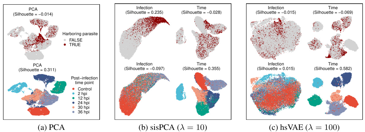
🔼 This figure compares the performance of PCA, sisPCA, and hsVAE in disentangling two sources of variation in scRNA-seq data: infection status and post-infection time. UMAP is used to visualize the high-dimensional data in two dimensions for each subspace. The color of each point represents the infection status (top row) or time point (bottom row). Ideally, the infection status would be clearly separated in the ‘infection’ subspace and less distinct in the ’time’ subspace; likewise, time points should be distinct in the ’time’ subspace but less so in the ‘infection’ subspace.
read the caption
Figure 5: UMAP visualizations of scRNA-seq data. Each column shows a different learned subspace: (a) PCA, (b) sisPCA-infection and sisPCA-time, and (c) hsVAE-infection and hsVAE-time. See Fig. 12 for other models. Cells are colored by either infection status (top row) or post-infection time (bottom row). In an optimal pair of subspaces, each property (infection status or time) should be more distinguishable in its corresponding subspace while showing less separation in the other.

🔼 This figure demonstrates the ability of sisPCA to recover latent subspaces in a simulated dataset. The ground truth contains three distinct 2D subspaces: one categorical, one continuous, and one unsupervised. The figure compares the performance of sisPCA and sPCA on this task. SisPCA is able to recover the underlying structure of the data more accurately than sPCA, demonstrating its ability to disentangle multiple latent subspaces.
read the caption
Figure 3: Example application of recovering a latent space with three subspaces (rows in panel a) embedded in a high-dimensional space. The first two subspaces (rows) of sPCA (panel b) and sisPCA (panel c) are supervised by the corresponding target variables.
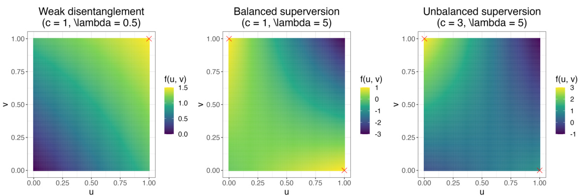
🔼 This figure demonstrates the ability of sisPCA to recover latent subspaces from high-dimensional data. Panel (a) shows the ground truth, with three distinct 2D subspaces (categorical, continuous, and unsupervised). Panel (b) shows the results of applying supervised PCA (sPCA), which fails to fully separate the subspaces. Panel (c) shows the results of applying sisPCA, which successfully separates the subspaces, even the unsupervised one, highlighting sisPCA’s ability to disentangle and interpret multiple factors in complex data.
read the caption
Figure 3: Example application of recovering a latent space with three subspaces (rows in panel a) embedded in a high-dimensional space. The first two subspaces (rows) of sPCA (panel b) and sisPCA (panel c) are supervised by the corresponding target variables.
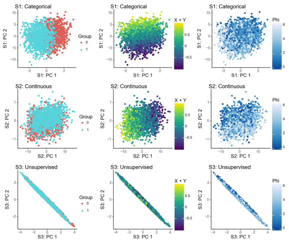
🔼 This figure demonstrates the performance of sisPCA and compares it to sPCA in recovering three subspaces embedded in a high dimensional space. The three subspaces represent different underlying data structures. The first two have associated target variables, allowing for supervised learning. The third subspace is unsupervised. The figure shows that sisPCA effectively separates the three subspaces, while sPCA struggles to disentangle them, particularly S2 and S3.
read the caption
Figure 3: Example application of recovering a latent space with three subspaces (rows in panel a) embedded in a high-dimensional space. The first two subspaces (rows) of sPCA (panel b) and sisPCA (panel c) are supervised by the corresponding target variables.

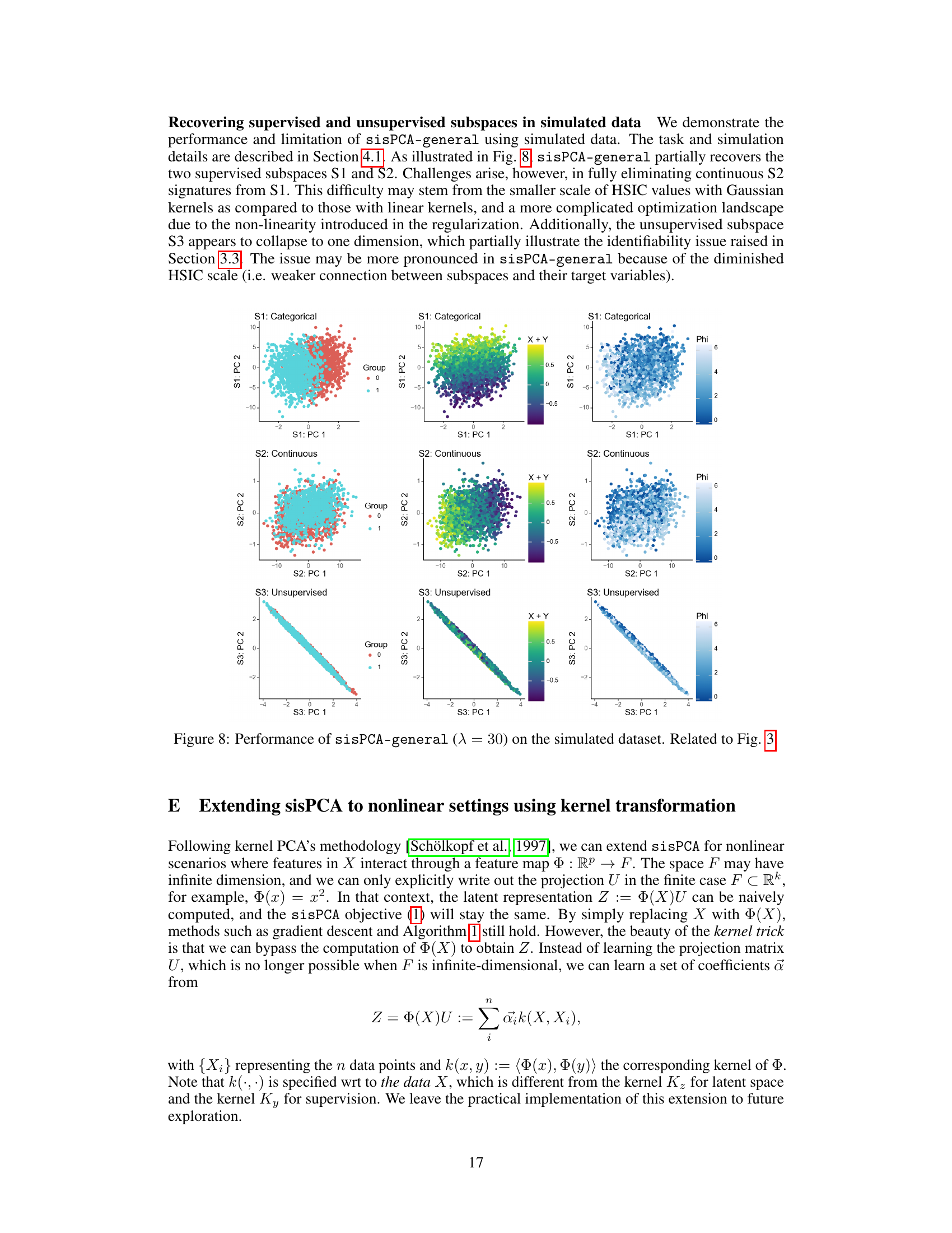
🔼 This figure demonstrates the effectiveness of sisPCA in recovering latent subspaces from high-dimensional data. Panel (a) shows the ground truth of three 2D subspaces with different characteristics (categorical, continuous, and unsupervised ring structure). Panel (b) displays the results obtained using supervised PCA (sPCA), showing that sPCA struggles to disentangle the subspaces, particularly failing to effectively recover the unsupervised subspace. In contrast, panel (c) presents the results obtained using sisPCA, showcasing its improved ability to disentangle the supervised subspaces and recover the unsupervised subspace’s underlying structure.
read the caption
Figure 3: Example application of recovering a latent space with three subspaces (rows in panel a) embedded in a high-dimensional space. The first two subspaces (rows) of sPCA (panel b) and sisPCA (panel c) are supervised by the corresponding target variables.

🔼 This figure shows how the disentanglement strength parameter λ affects the learned subspaces in the breast cancer dataset analysis. It presents a grid of plots, each showing a 2D UMAP projection of the ‘symmetry’ subspace for a different value of λ. The plots visualize the separation of benign and malignant samples within the subspace. The heatmap shows the pairwise similarity between models trained with different λ values. A loss curve shows how the reconstruction loss and regularization loss vary with λ, indicating convergence to a robust solution.
read the caption
Figure 9: Effect of λ on the learned subspace structure in the breast cancer dataset. Related to Fig. 4.

🔼 This figure shows the impact of the hyperparameter λ (lambda_contrast) on the learned subspaces in the breast cancer dataset analysis. The left panel displays the pairwise similarity between sisPCA models with different λ values, showing a clear separation of the sPCA solution (λ=0) from other models. As λ increases, the symmetry subspace becomes less predictive of the diagnostic status (middle panel), while the subspaces stabilize after λ=1 (right panel). The convergence pattern is also reflected in the elbow of the reconstruction loss curve (bottom right panel).
read the caption
Figure 9: Effect of λ on the learned subspace structure in the breast cancer dataset. Related to Fig. 4.

🔼 This figure shows the effect of the hyperparameter λ (disentanglement strength) on the learned subspaces of the single-cell malaria infection data. The top row displays the infection subspace colored by infection status (TRUE/FALSE), and the bottom row shows the same subspace colored by time point. Each column represents a different value of λ. The results suggest that as λ increases, the separation between infected and uninfected cells becomes clearer in the infection subspace, while the temporal variations become less pronounced. This indicates that the model successfully disentangles the biological processes related to infection status from the temporal dynamics of infection.
read the caption
Figure 10: Effect of λ on the learned subspace structure in the single-cell malaria infection data. Related to Fig. 5 and Fig. 6.
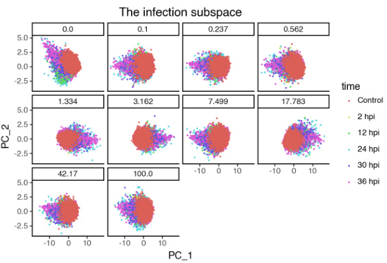
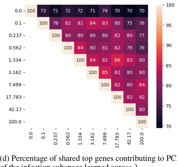
🔼 This figure visualizes the effect of the hyperparameter λ (disentanglement strength) on the learned subspaces in the single-cell malaria infection analysis. It shows how the separation of infected and uninfected cells, as well as the separation of different time points post-infection, changes with increasing λ. Panels (a) and (b) show UMAP projections of the infection subspace colored by infection status and time point, respectively, for different values of λ. Panel (c) displays a heatmap showing the similarity between the subspaces for different values of λ. Panel (d) shows the percentage of shared top genes contributing to PC1 of the infection subspace across different values of λ. The results illustrate the impact of λ on the ability of sisPCA to disentangle relevant biological signals.
read the caption
Figure 10: Effect of λ on the learned subspace structure in the single-cell malaria infection data. Related to Fig. 5 and Fig. 6.
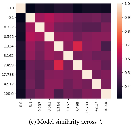
🔼 This figure shows the effect of the hyperparameter λ (disentanglement strength) on the learned subspaces in a single-cell RNA sequencing dataset of malaria infection. Panel (a) and (b) display UMAP visualizations of the infection subspace colored by infection status and time point, respectively, for various values of λ. The heatmaps in (c) and (d) show the model similarity (in terms of shared top genes contributing to PC1 of the infection subspace) across different values of λ. The results demonstrate that increased λ leads to better separation of infection status and time point effects in the infection subspace.
read the caption
Figure 10: Effect of λ on the learned subspace structure in the single-cell malaria infection data. Related to Fig. 5 and Fig. 6.
🔼 This figure compares the performance of sPCA and sisPCA in recovering three latent subspaces embedded in a high-dimensional space. The ground truth (panel a) shows three distinct subspaces: one categorical, one continuous, and one unsupervised. sPCA (panel b) fails to completely separate the subspaces, particularly mixing the continuous subspace with the other two. sisPCA (panel c) more effectively disentangles the subspaces, accurately representing the underlying structure of each. The first two subspaces in both sPCA and sisPCA are supervised by corresponding target variables, highlighting sisPCA’s ability to incorporate supervision for better subspace separation and interpretability.
read the caption
Figure 3: Example application of recovering a latent space with three subspaces (rows in panel a) embedded in a high-dimensional space. The first two subspaces (rows) of sPCA (panel b) and sisPCA (panel c) are supervised by the corresponding target variables.
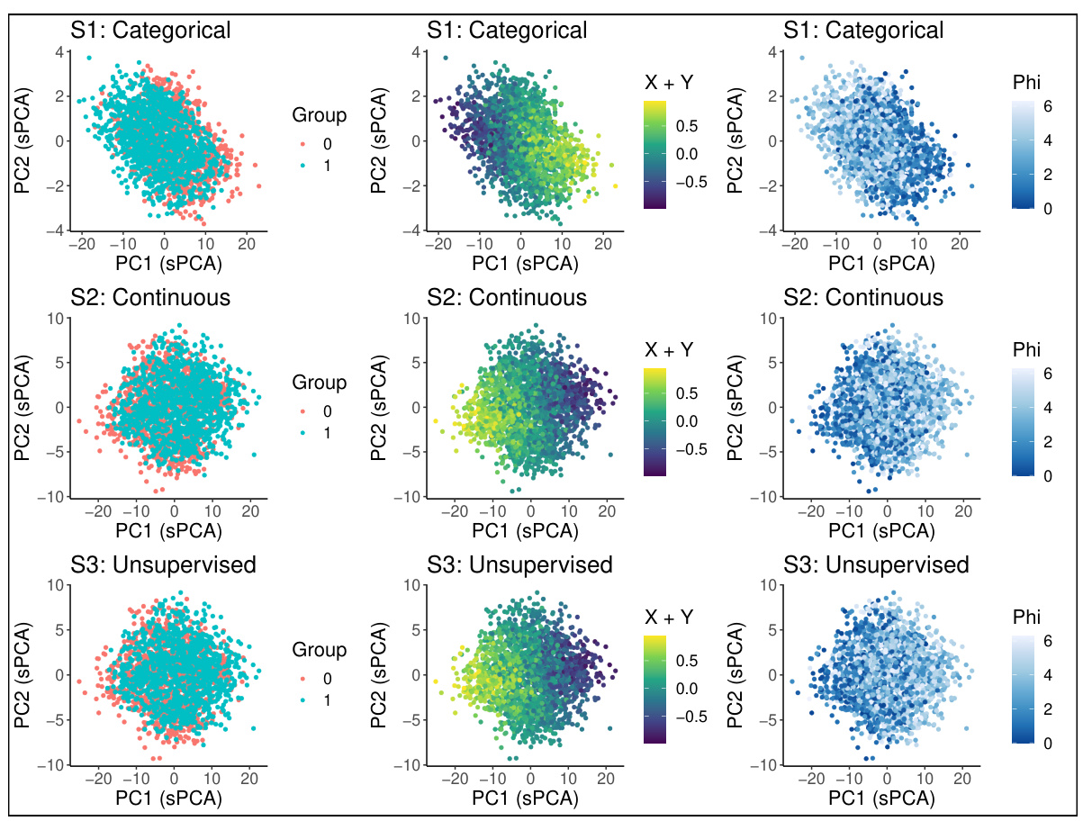
🔼 This figure demonstrates the performance of sisPCA in recovering latent subspaces compared to sPCA. The ground truth is shown in (a), showing three subspaces: one categorical, one continuous, and one unsupervised. sPCA (b) fails to clearly separate the subspaces, especially the unsupervised one, which is heavily influenced by the continuous subspace’s variability. sisPCA (c) successfully disentangles the three subspaces, showing distinct patterns for each and recovering the circular structure of the unsupervised subspace.
read the caption
Figure 3: Example application of recovering a latent space with three subspaces (rows in panel a) embedded in a high-dimensional space. The first two subspaces (rows) of sPCA (panel b) and sisPCA (panel c) are supervised by the corresponding target variables.
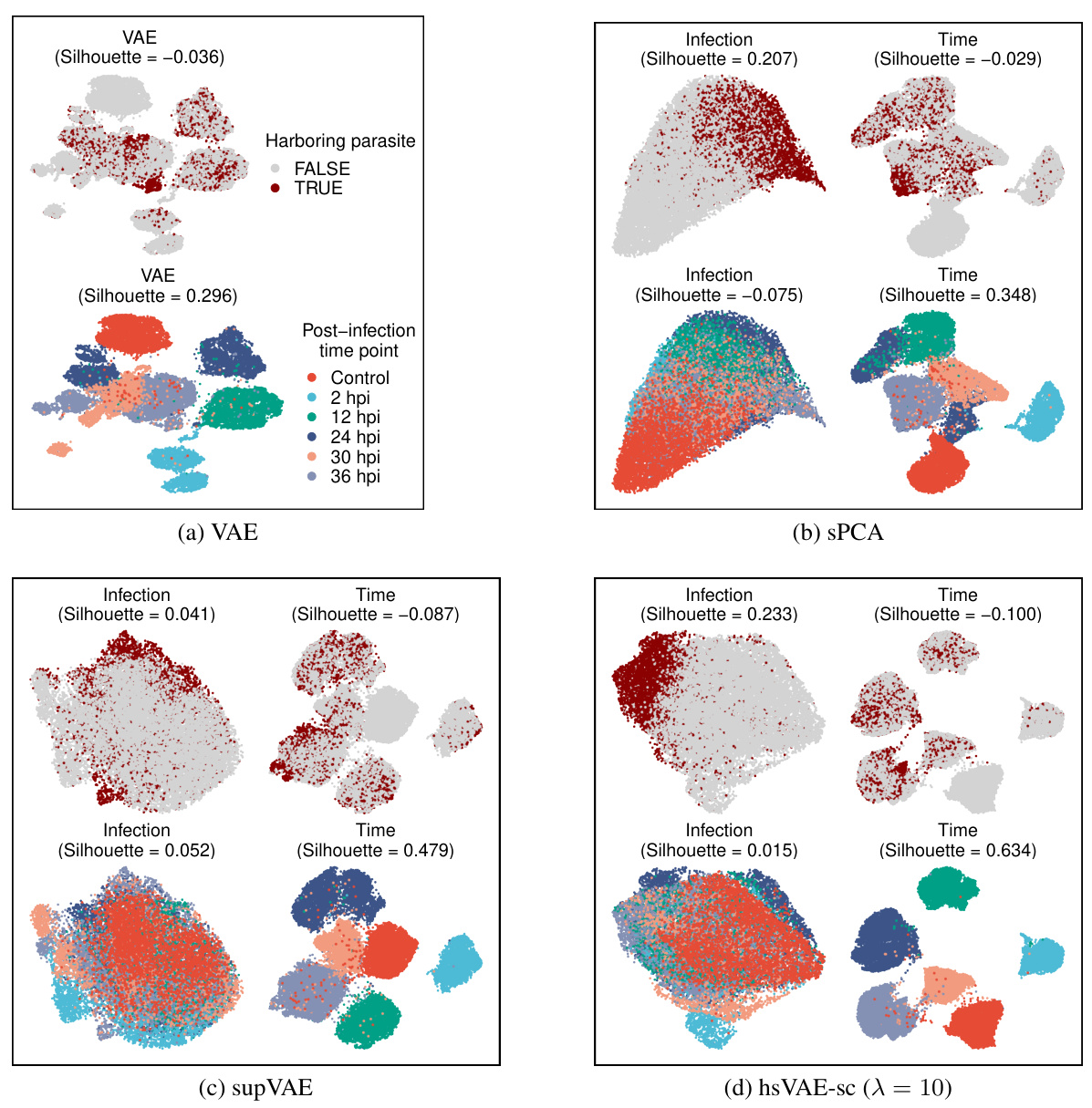
🔼 This figure compares the performance of different dimensionality reduction techniques (VAE, sPCA, supVAE, and hsVAE-sc) on scRNA-seq data of mouse liver infected with Plasmodium. It visualizes the learned subspaces using UMAP, showing how well each method separates infected/uninfected cells and separates cells based on the post-infection time. The results highlight sisPCA’s (hsVAE-sc) superior ability to disentangle infection status and time effects compared to other methods.
read the caption
Figure 12: UMAP visualizations of the scRNA-seq data of mouse liver upon Plasmodium infection. Subspace representations are learned using unsupervised VAE (a) and supervised sPCA (b), supVAE (c) and hsVAE-sc (d). Note that the infection subspaces of VAE and supVAE fail to distinguish infected versus uninfected cells. Moreover, all infection subspaces presented here still exhibit significant temporal patterns (lower left plot in each panel) where cells collected at different time points are not fully mixed.
More on tables

🔼 This table presents the information density for each subspace obtained by PCA, sPCA and sisPCA with different regularization strengths (λ). The information density is measured using the maximum Spearman correlation with age and the Silhouette score with cancer type. The results show how the different methods and regularization parameters affect the ability to separate information related to aging and cancer in the different subspaces.
read the caption
Table 2: Information density in each sisPCA subspace.

🔼 This table quantitatively evaluates the quality of subspace representations learned by different models (PCA, sPCA, sisPCA, VAE, supVAE, hsVAE) on a scRNA-seq dataset. It uses two metrics: Grassmann distance, measuring the separation between subspaces, and silhouette score, evaluating the quality of clustering within each subspace for both infection status and time points. Higher Grassmann distance indicates better subspace separation. Higher silhouette scores signify better-defined clusters. The results show that sisPCA achieves a good balance between subspace separation and cluster quality.
read the caption
Table 3: Quantitative evaluation of subspace representation quality.
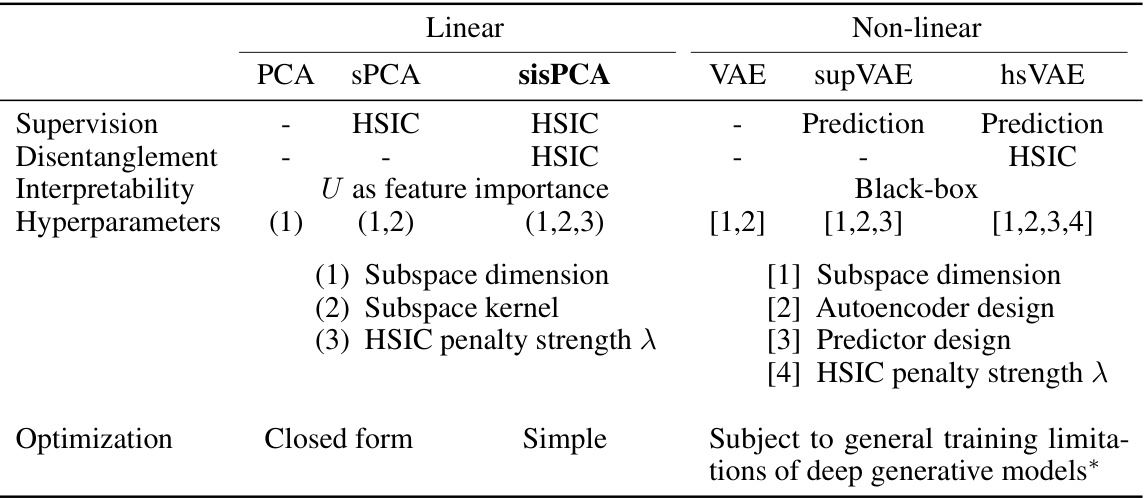
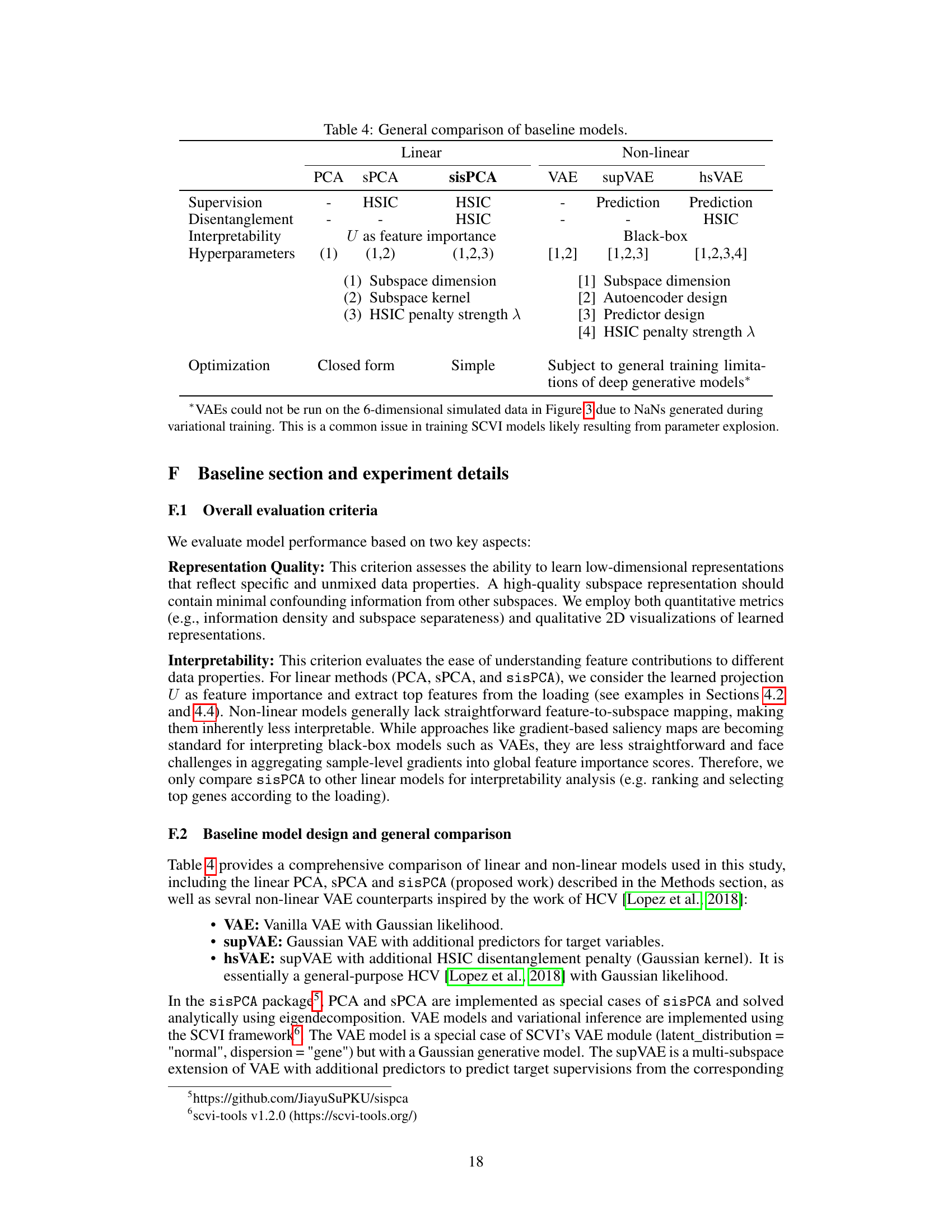
🔼 This table compares several baseline models used in the paper, including PCA, sPCA, sisPCA, VAE, supVAE, and hsVAE. It contrasts their approaches to supervision (none, HSIC-based, prediction), disentanglement (none, HSIC-based), interpretability (linear projection features vs. black box), hyperparameters (number and type), and optimization methods (closed-form, simple iterative, or complex deep learning). The table highlights the trade-offs between model complexity, interpretability, and performance.
read the caption
Table 4: General comparison of baseline models.
Full paper#

