↗ OpenReview ↗ NeurIPS Homepage ↗ Chat
TL;DR#
Community detection, crucial for understanding network structures, traditionally relies on objective functions optimized by custom algorithms. However, these methods often lag behind recent advancements in deep learning. This paper addresses this limitation.
The paper introduces Neuromap, a novel approach that integrates the map equation, a well-regarded information-theoretic objective function, into a differentiable framework suitable for optimization using gradient descent and graph neural networks (GNNs). This allows for end-to-end learning, automatic cluster number selection, and the incorporation of node features. Neuromap’s performance is competitive against other deep graph clustering methods, showcasing the benefits of combining traditional network science techniques with deep learning.
Key Takeaways#
Why does it matter?#
This paper is important because it bridges the gap between network science and deep learning for community detection. By making the map equation, a popular information-theoretic approach, compatible with neural networks, it offers a novel and powerful technique. This opens up new avenues for research, particularly in handling large-scale datasets and incorporating node features effectively, leading to improved accuracy and efficiency in community detection.
Visual Insights#

This figure illustrates the coding principles behind the map equation used for community detection. It compares two scenarios: one where all nodes belong to a single module (left), requiring longer codewords, and another where nodes are partitioned into modules (right), allowing for shorter codewords by reusing them. The middle part shows the two encodings for comparison. The figure demonstrates how community detection, via the map equation, essentially reduces to a compression problem.
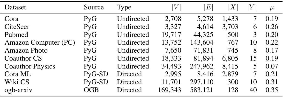
This table lists properties of ten real-world network datasets used in the paper’s experiments. For each dataset, it provides the source, type (directed or undirected), number of nodes (|V|), number of edges (|E|), node feature dimension (|X|), number of communities (|Y|), and mixing parameter (μ). The mixing parameter indicates the proportion of edges that connect nodes within different communities, with higher values signifying more overlap between communities.
In-depth insights#
Neuromap: Map Equation#
The heading ‘Neuromap: Map Equation’ suggests a novel approach to community detection in networks. Neuromap likely represents a neural network-based algorithm, leveraging the strengths of deep learning to optimize the map equation. The map equation, a well-established information-theoretic method, quantifies the efficiency of describing network flow through community structures. Combining this with a neural network architecture (Neuromap) likely allows for end-to-end learning, automatic cluster identification, and the seamless integration of node features. This approach potentially surpasses traditional map equation optimization techniques by offering greater scalability and accuracy, particularly in complex, large-scale networks. The differentiable formulation of the map equation within Neuromap is crucial, enabling gradient-based optimization and potentially superior performance to other deep graph clustering methods. The name ‘Neuromap’ itself cleverly hints at a connection between the established Infomap algorithm and the novel neural network implementation. Overall, this innovative fusion of classic network science with modern deep learning promises significant advancement in the field of community detection.
GNN for Clustering#
Graph Neural Networks (GNNs) have emerged as powerful tools for graph-structured data analysis, and their application to clustering problems is a rapidly developing area. GNNs excel at capturing both the topological structure of the graph and node features, which are crucial aspects for effective clustering. Unlike traditional clustering algorithms, GNNs can learn complex, non-linear relationships between nodes, leading to more accurate and nuanced cluster assignments. A key advantage is the ability of GNNs to handle large-scale datasets that are intractable for many conventional methods. However, challenges remain, including the computational cost of training deep GNNs and the interpretability of the learned representations. Furthermore, the selection of the optimal GNN architecture and hyperparameters is crucial for achieving good performance, and requires careful consideration. Research is ongoing to improve the efficiency, scalability, and interpretability of GNN-based clustering techniques, aiming to further leverage the unique strengths of GNNs for tackling challenging clustering problems in various domains.
Synthetic Tests#
In evaluating community detection methods, synthetic tests using computer-generated networks play a crucial role. These tests offer the advantage of known ground truth, allowing for precise evaluation of algorithm performance. By systematically varying network parameters like size, density, and community structure, researchers gain valuable insights into an algorithm’s strengths and weaknesses under controlled conditions. LFR benchmark networks, for example, are frequently used because of their ability to mimic real-world networks’ characteristics, including power-law degree distributions. Through comparison to baselines and varying mixing parameters, synthetic tests provide a quantitative assessment of performance. However, it’s important to note that synthetic tests may not fully capture the complexities and nuances of real-world networks. While they provide a controlled environment, they lack the noise and irregularities present in real-world data, potentially leading to over-optimistic performance evaluations.
Real-World Data#
When evaluating community detection methods, the use of real-world data is crucial for assessing practical performance and generalizability. Real-world networks are inherently more complex than synthetic datasets, exhibiting characteristics like noise, sparsity, and potentially unknown ground truth community structures. This complexity challenges the assumptions of many algorithms optimized on idealized synthetic data. Therefore, analyzing results on real-world networks provides a more robust and reliable evaluation of the algorithm’s strengths and limitations in handling realistic scenarios. The selection of real-world datasets should be diverse and representative of various domains and network structures. Careful consideration must be given to the characteristics of each dataset (size, density, presence of node features, etc.), its limitations and potential biases, and how those might affect the performance metrics. The existence of ‘ground truth’ community structures in real-world datasets is often debated. The absence of a definitive ground truth necessitates using alternative evaluation metrics that are robust to the uncertainties present in real-world data. Furthermore, comparing performance on multiple real-world datasets, alongside a thorough analysis of the results, will offer a comprehensive evaluation of a community detection algorithm’s ability to generalize to various data characteristics. This should include discussion of whether the results hold consistently across different network types, sizes, and properties.
Future of Neuromap#
The future of Neuromap looks promising, given its strong performance in community detection. Further research could focus on enhancing its scalability to handle even larger, more complex networks, perhaps through exploring more efficient graph neural network architectures or distributed computing techniques. Extending Neuromap to incorporate temporal dynamics within networks would be a valuable advancement, allowing for the analysis of evolving community structures over time. Investigating applications beyond graph clustering is another exciting avenue, such as node classification or link prediction, leveraging Neuromap’s ability to capture community structure. Finally, in-depth theoretical analysis of Neuromap’s capabilities and limitations, particularly concerning the impact of different network characteristics on its performance, will solidify its position as a leading method in community detection.
More visual insights#
More on figures
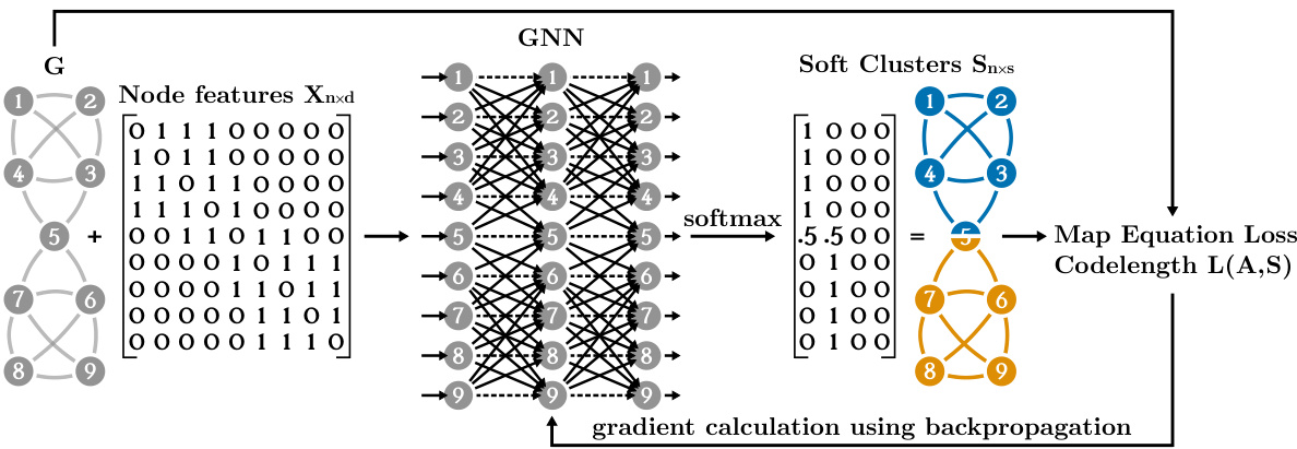
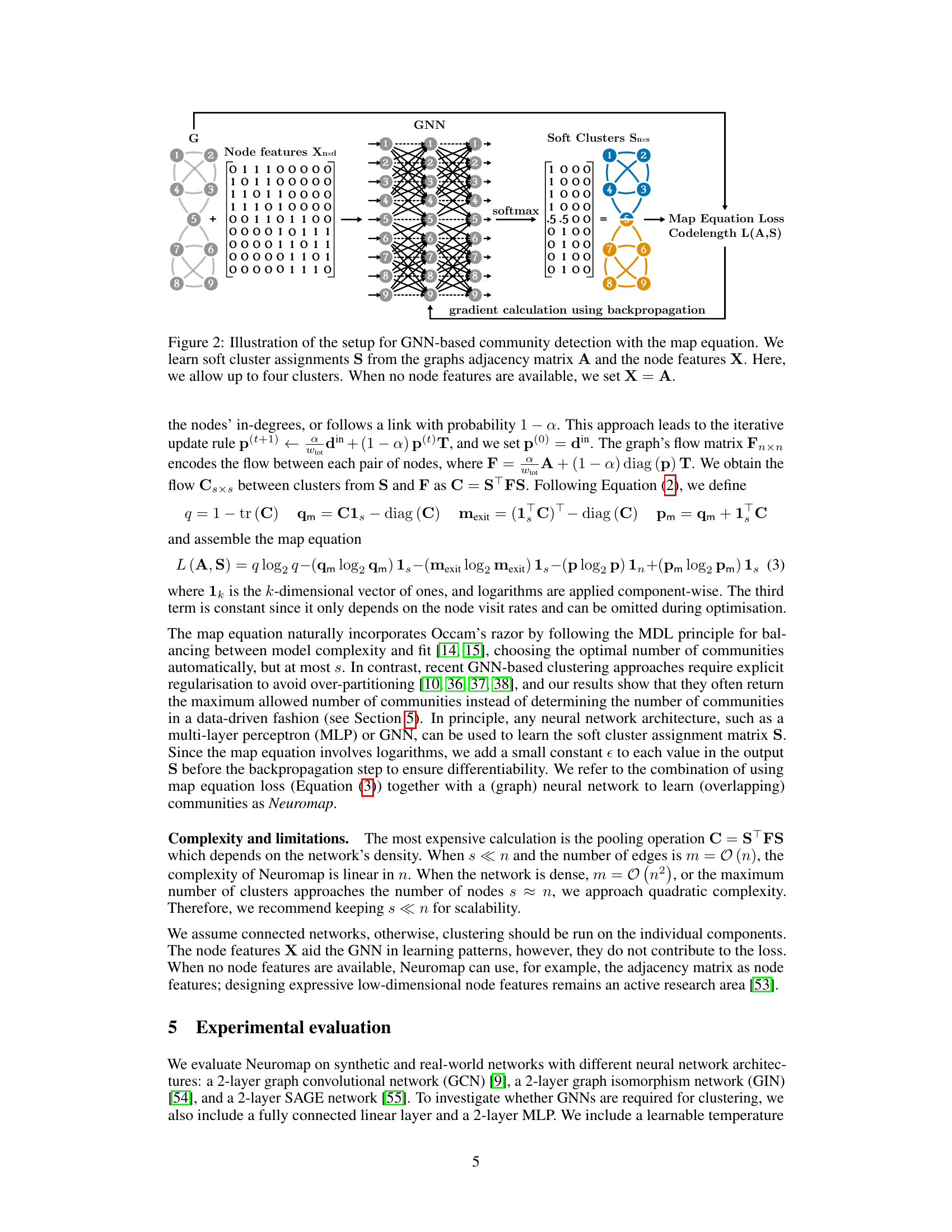
This figure illustrates the process of community detection using graph neural networks and the map equation. A graph neural network (GNN) takes the graph’s adjacency matrix (A) and node features (X) as input. The GNN processes this information to produce a soft cluster assignment matrix (S), which represents the probability of each node belonging to each of the s clusters (maximum 4 in this example). This matrix S is then used to compute the codelength, L(A,S), via the map equation. The goal is to minimize this codelength through backpropagation, effectively learning optimal cluster assignments. When node features are unavailable, the adjacency matrix is used as a substitute for node features.
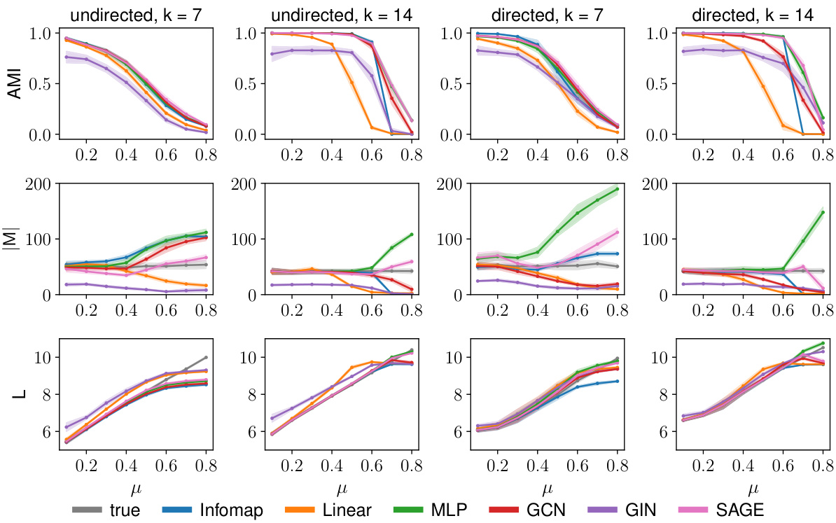
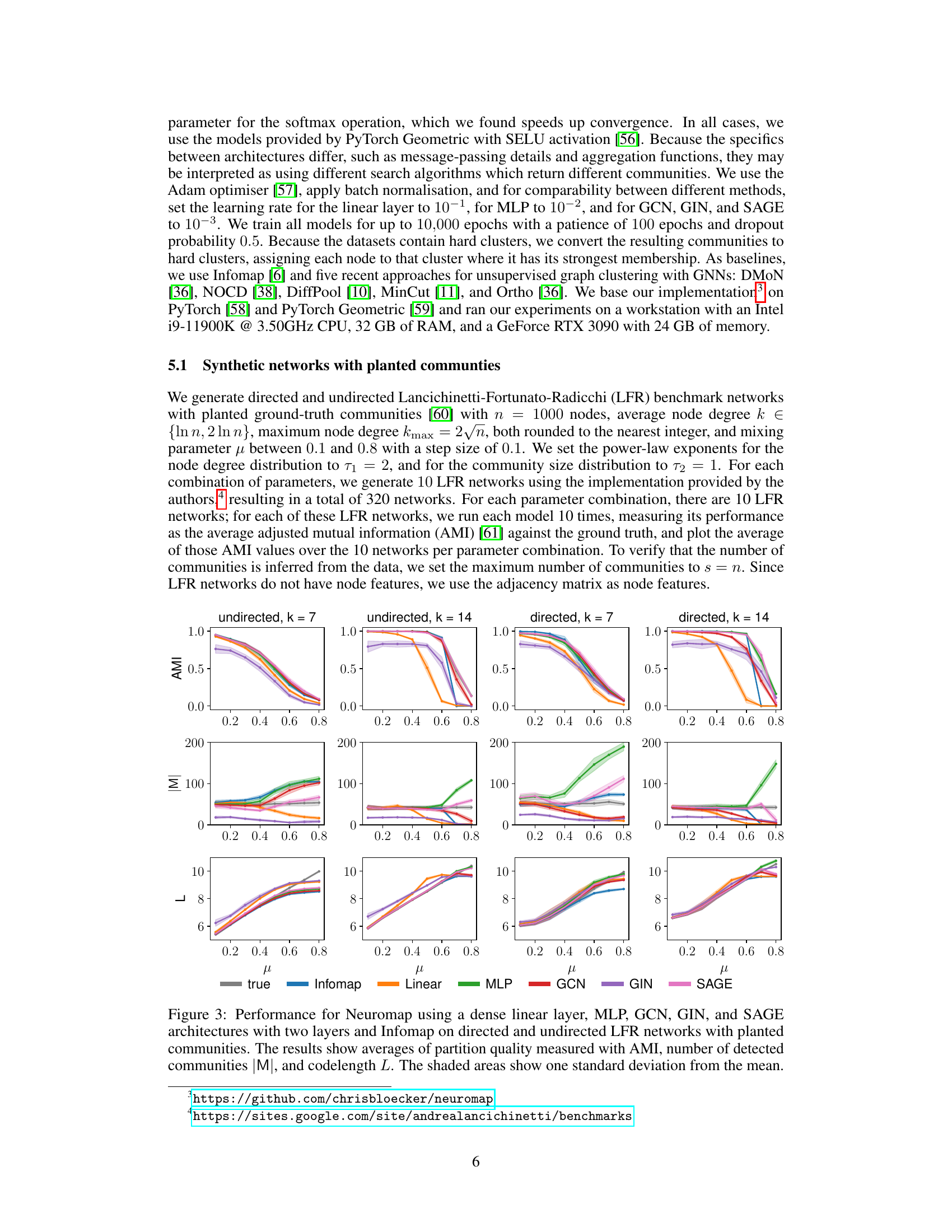
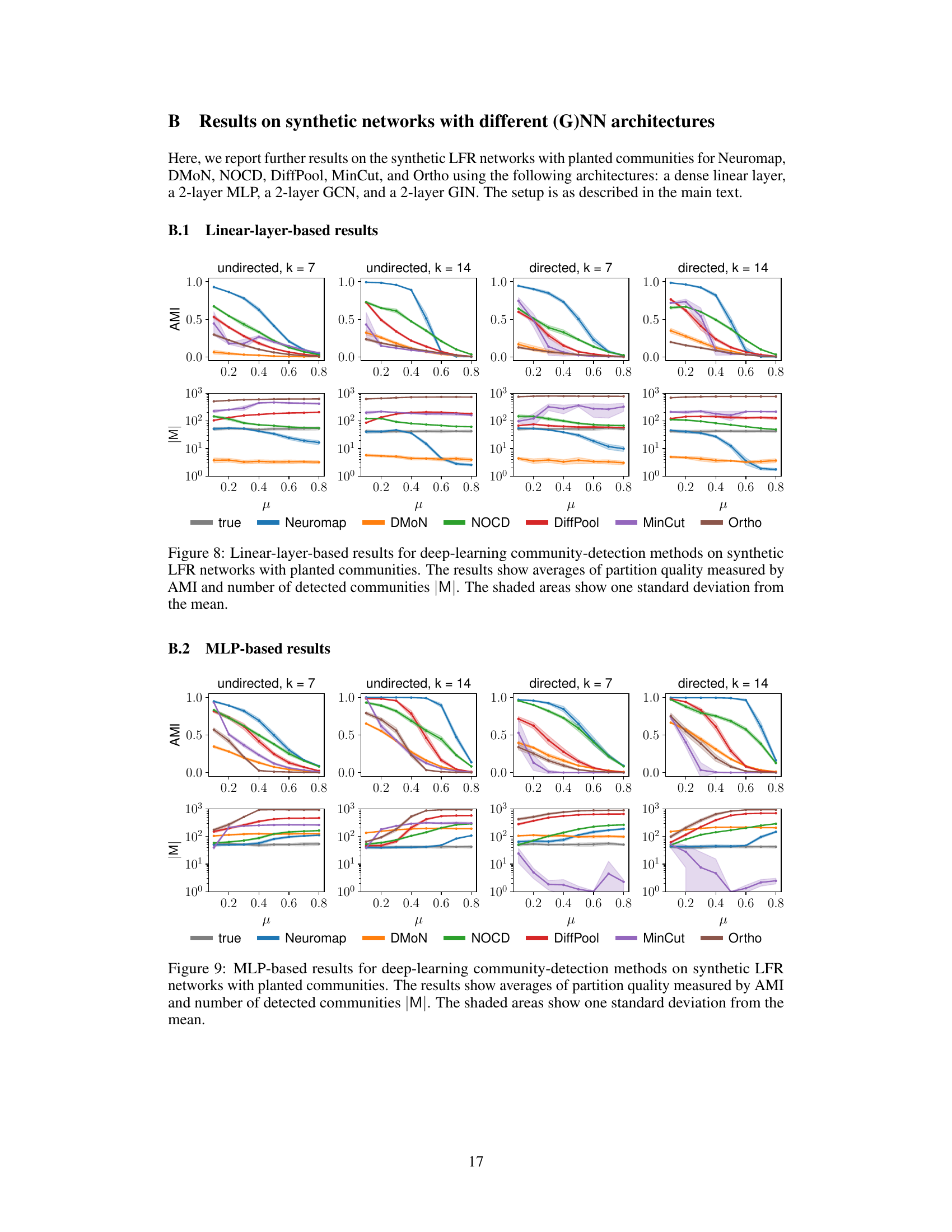
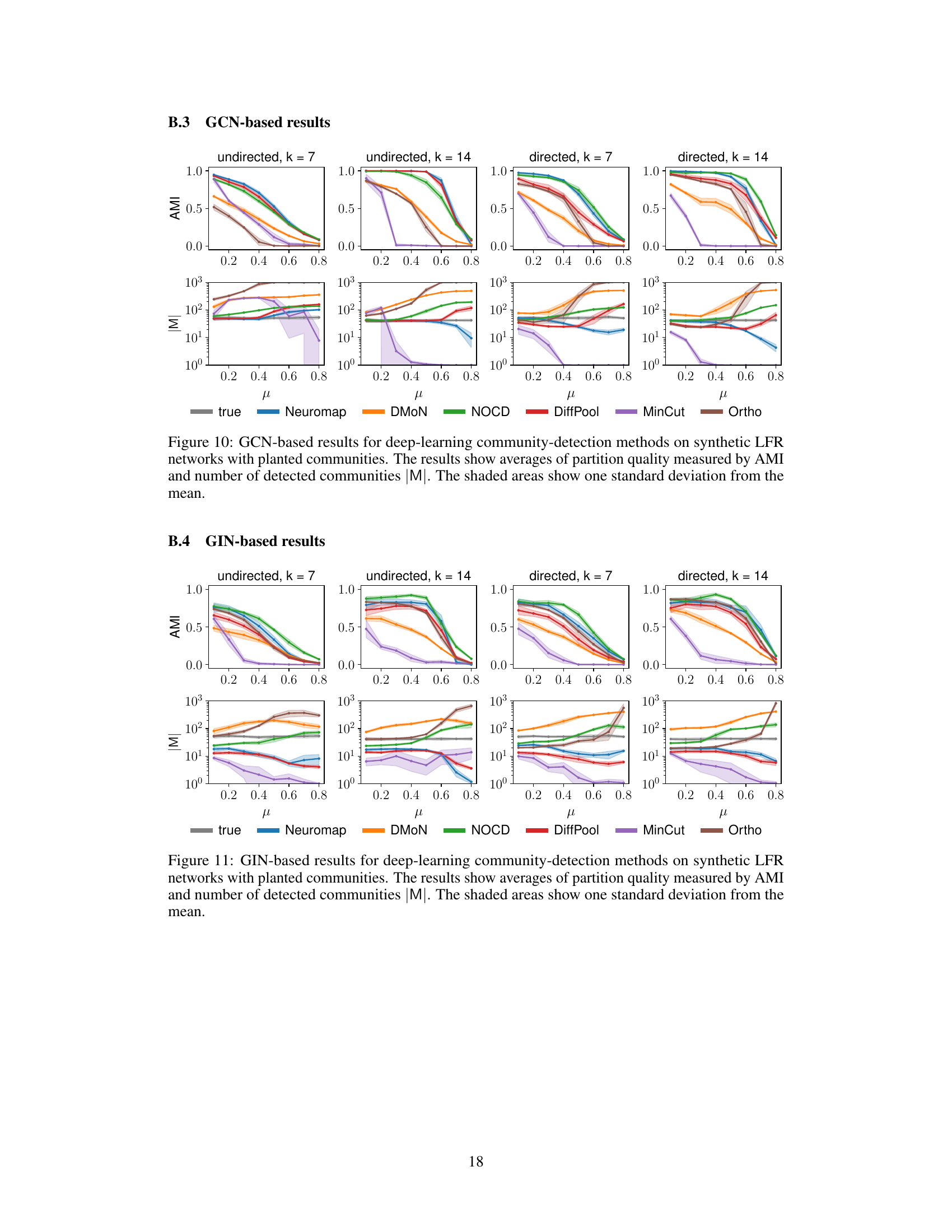
This figure displays the performance of Neuromap (using different neural network architectures) and Infomap on directed and undirected LFR benchmark networks with planted communities. The performance is evaluated using three metrics: Adjusted Mutual Information (AMI), the number of detected communities (|M|), and the codelength (L). Higher AMI values indicate better performance. The shaded areas represent one standard deviation from the mean, illustrating variability in the results. The x-axis represents the mixing parameter (μ) which controls the amount of noise or randomness in the network structure.
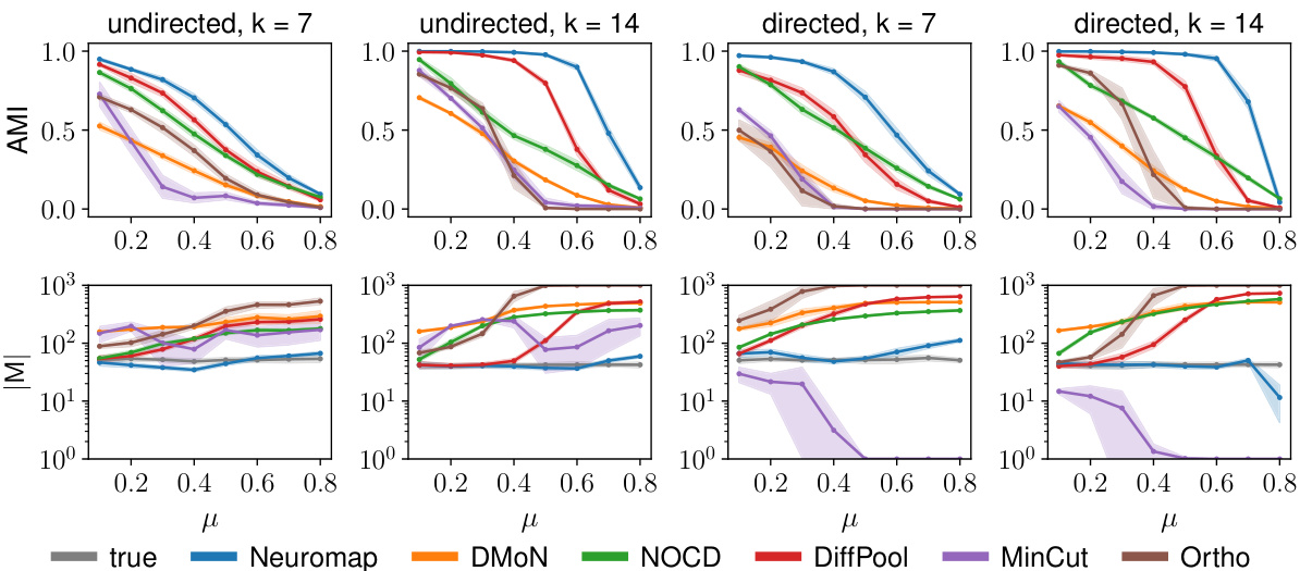
This figure displays the performance comparison of Neuromap (with different neural network architectures) and Infomap on directed and undirected LFR benchmark networks. The x-axis represents the mixing parameter (μ), and the y-axis shows three different metrics: Adjusted Mutual Information (AMI), the number of detected communities (M), and the codelength (L). Each metric’s average value and standard deviation are shown for various μ values. The plot helps to assess Neuromap’s performance against a well-established baseline.
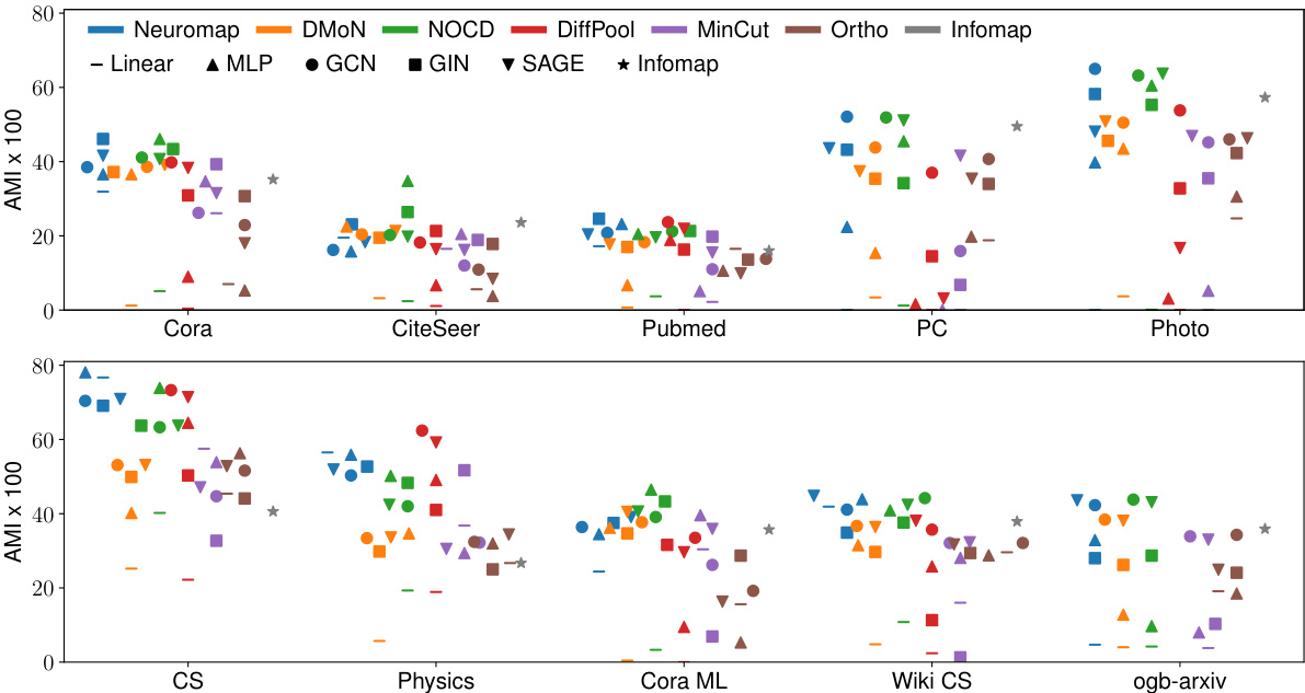
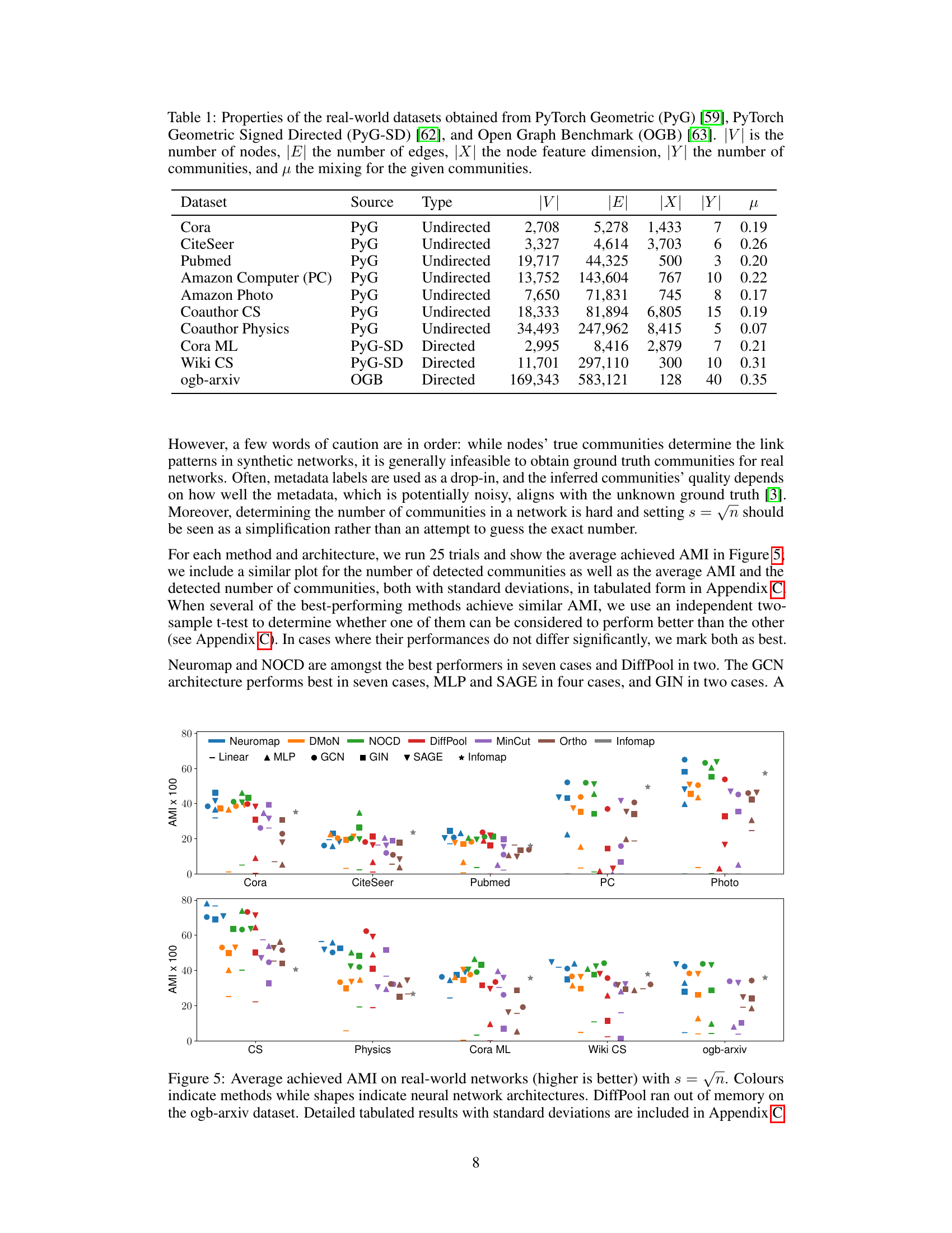
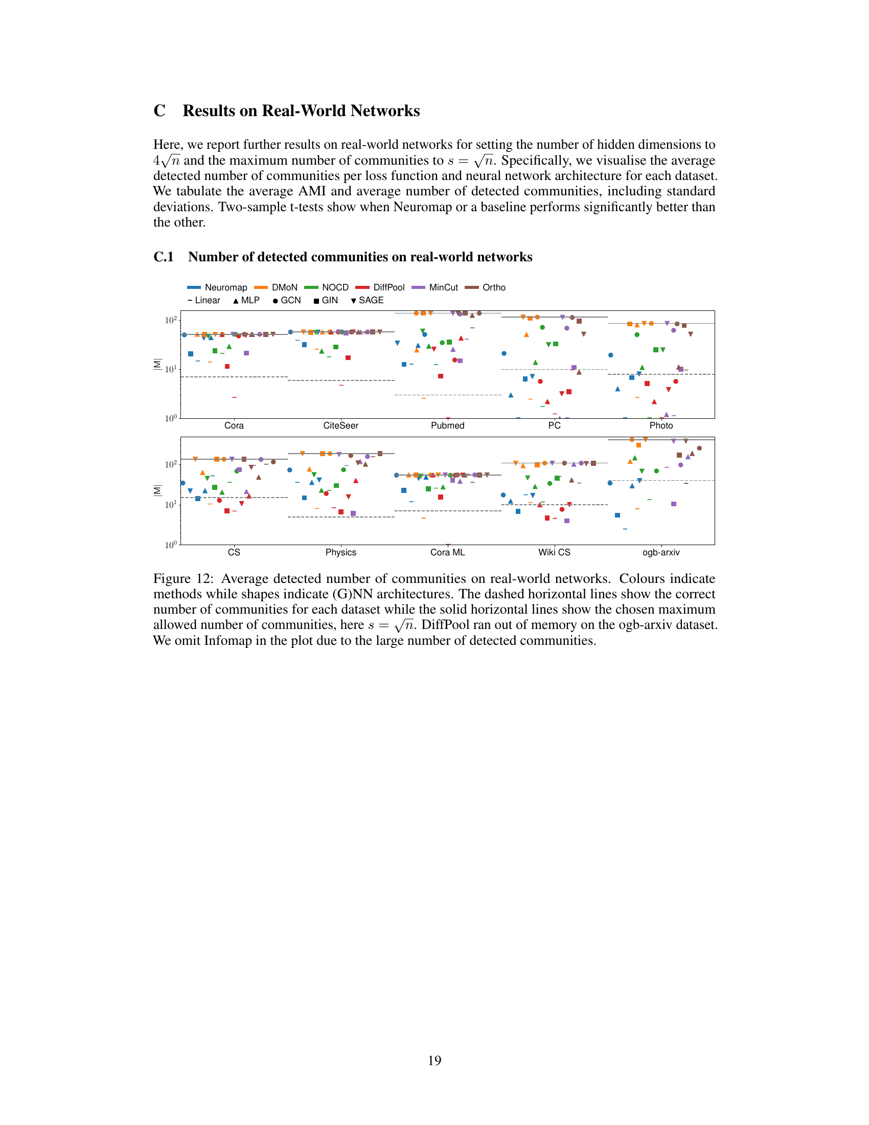
This figure compares the performance of Neuromap and several baseline methods on ten real-world datasets, where each node has multiple features. The x-axis represents the datasets, and the y-axis represents the average Adjusted Mutual Information (AMI) score. The AMI score measures the similarity between the detected communities and the ground truth communities. The higher the score, the better. Different shapes represent various neural network architectures (Linear, MLP, GCN, GIN, and SAGE) and Neuromap. A dashed horizontal line indicates the maximum allowed number of communities, which is set to √n. The figure shows that Neuromap achieves comparable or better performance in many datasets compared to the baseline methods and that the performance depends on the specific dataset and neural network architecture used. DiffPool failed on one dataset due to memory constraints.
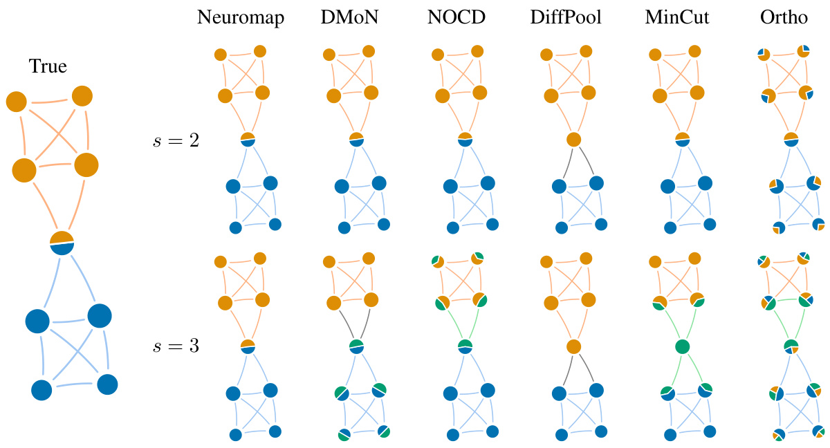
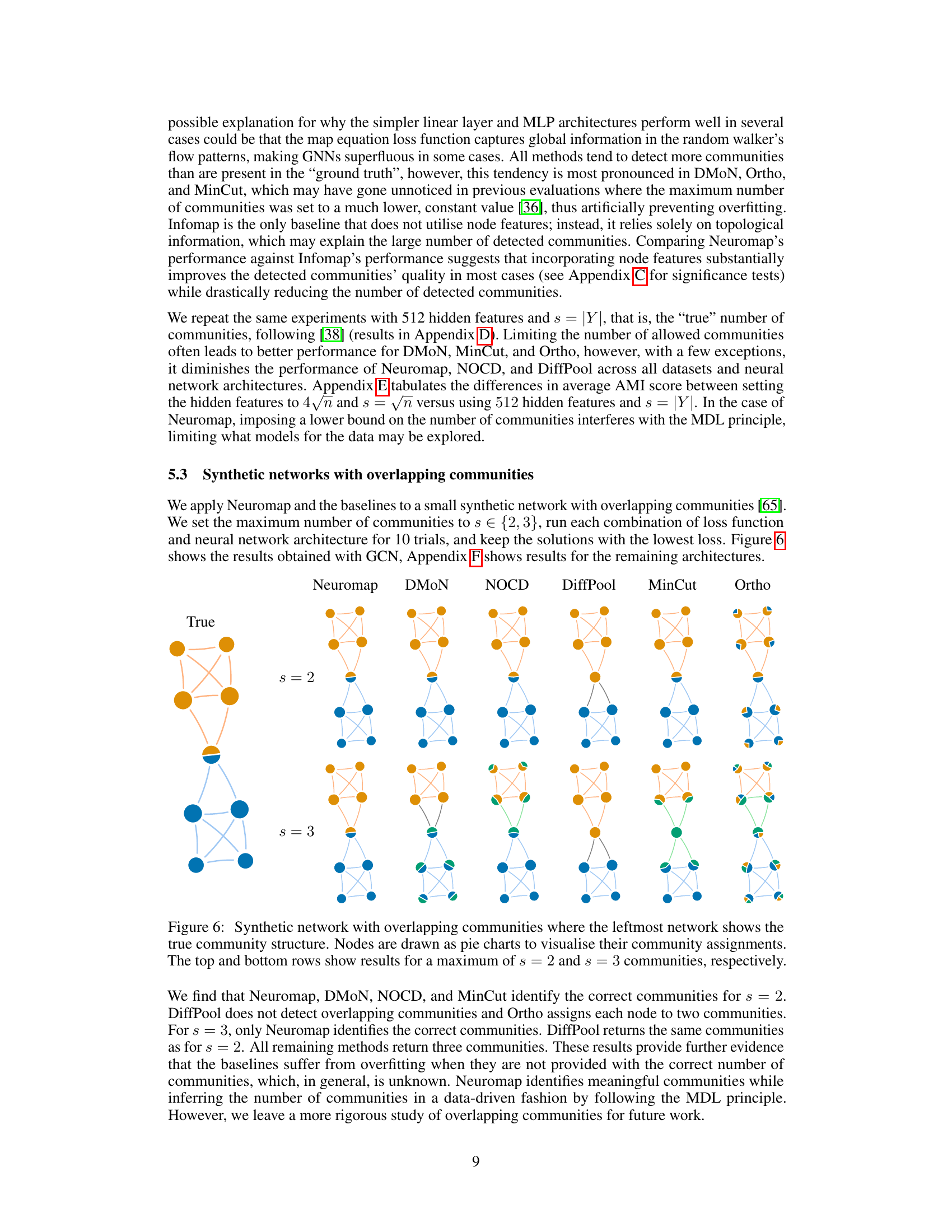
This figure displays results from various community detection methods on a small synthetic network with overlapping communities. The leftmost graph represents the ground truth, showing the true community assignments of each node. The remaining graphs illustrate the results obtained from different methods (Neuromap, DMON, NOCD, DiffPool, MinCut, Ortho) for two different maximum numbers of communities (s=2 and s=3). Each node is depicted as a pie chart, with the proportions of the segments representing its assignment to the detected communities. This visualization helps compare how accurately each method identifies and represents overlapping community structures.
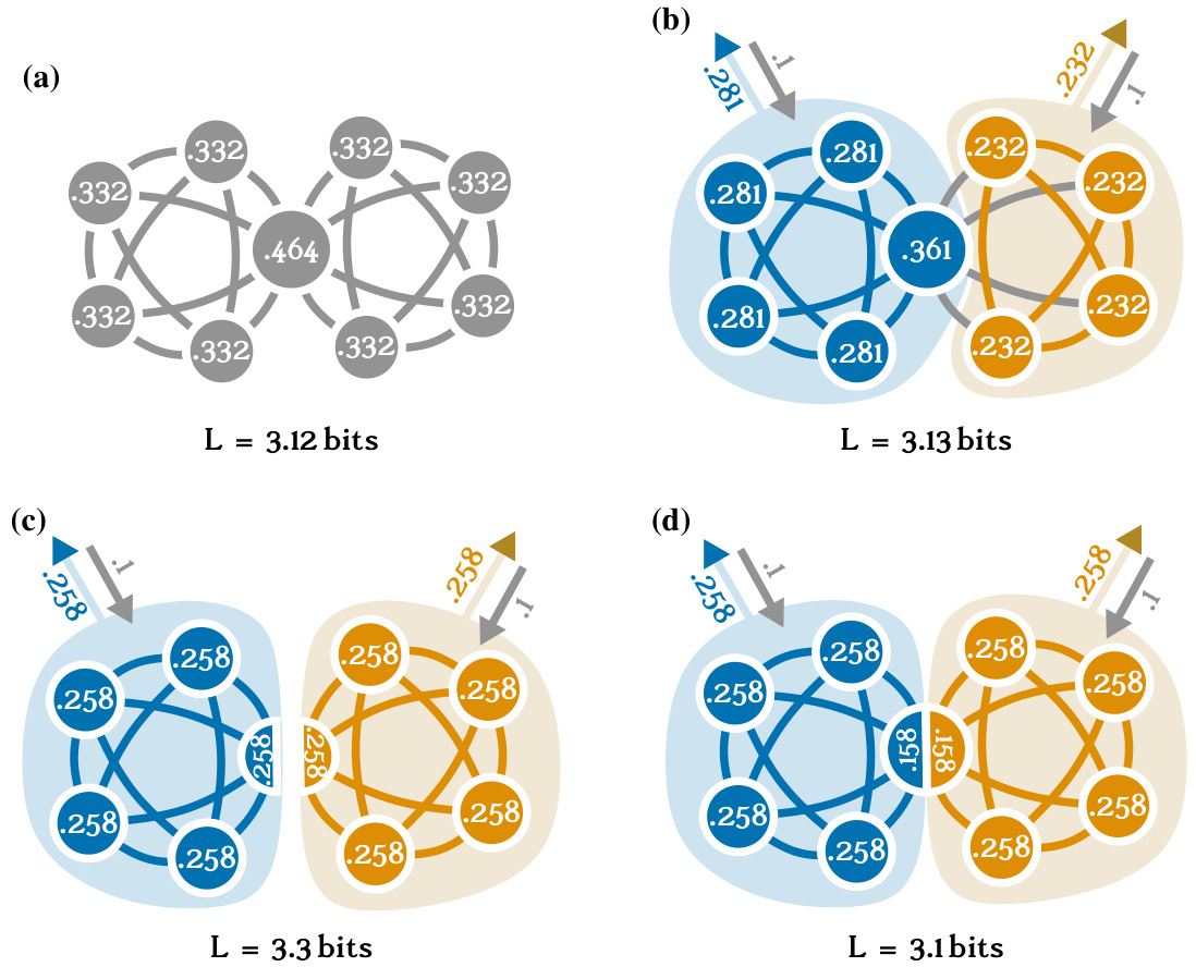
This figure illustrates the coding principles behind the map equation used for community detection. The left panel shows a network where all nodes belong to a single module, resulting in a longer codeword length (60 bits) to encode random walks. The right panel shows the same network partitioned into modules, allowing for codeword reuse and a shorter codeword length (48 bits). The middle panel highlights the difference in encoding schemes between the two scenarios.
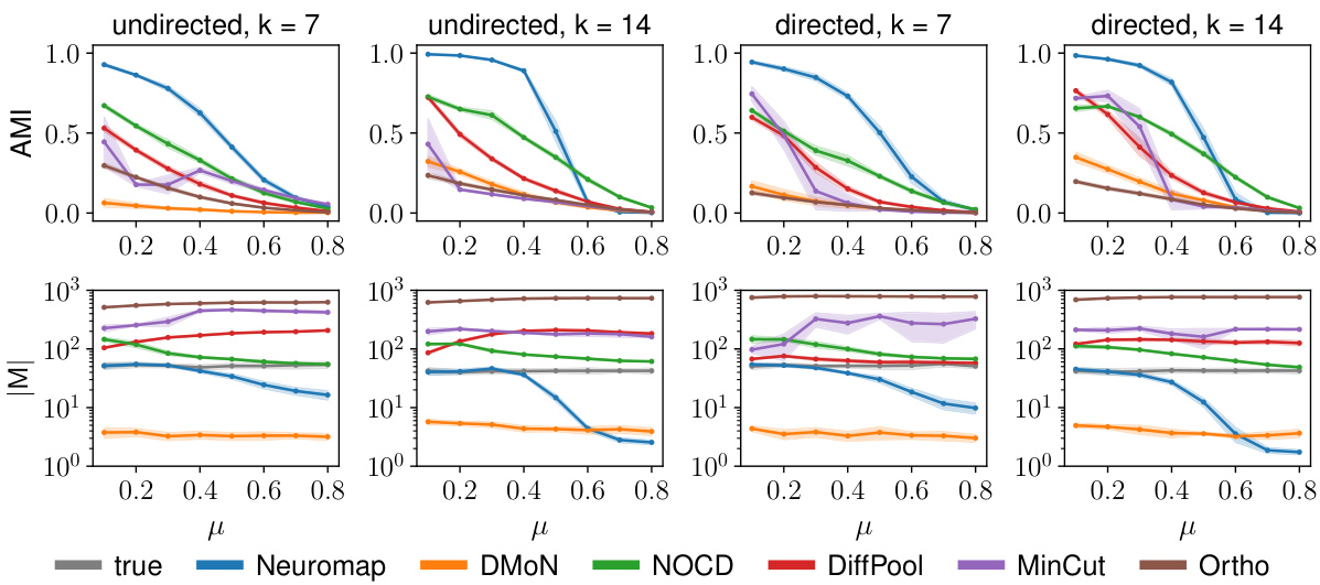
This figure presents the performance comparison of Neuromap (using different neural network architectures: dense linear layer, MLP, GCN, GIN, and SAGE) and Infomap on synthetic LFR networks with planted communities. The performance is evaluated using three metrics: Adjusted Mutual Information (AMI) to assess the quality of community detection; the number of detected communities (M); and the codelength (L) representing the description length of the random walk. The shaded regions indicate standard deviations. The x-axis represents the mixing parameter (μ), illustrating the transition between communities.
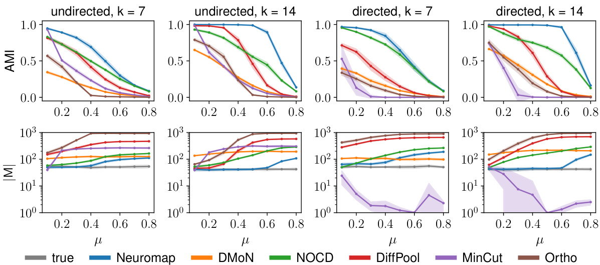
This figure displays the performance comparison between different neural network architectures (dense linear layer, MLP, GCN, GIN, and SAGE) and Infomap for community detection on synthetic LFR networks. The evaluation metrics include the Adjusted Mutual Information (AMI) score, the number of detected communities (M), and the codelength (L). Higher AMI values indicate better clustering performance. The shaded regions represent one standard deviation from the mean across multiple trials, indicating the variability of results. The figure illustrates how different architectures handle communities under varying mixing parameter (μ) values and different average degree values.
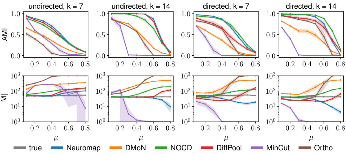
This figure compares the performance of Neuromap using various neural network architectures (dense linear layer, MLP, GCN, GIN, and SAGE) against Infomap on both directed and undirected LFR benchmark networks. The x-axis represents the mixing parameter (μ) of the LFR networks, which controls the strength of community structure. The top row shows the Adjusted Mutual Information (AMI), a metric measuring the similarity between the detected and the ground-truth community structures. The bottom row displays the number of communities detected (|M|) and the codelength (L). The shaded regions indicate standard deviations across multiple runs for each model. The figure aims to demonstrate Neuromap’s ability to accurately detect communities in networks with varying levels of community structure, even when using different neural network architectures.
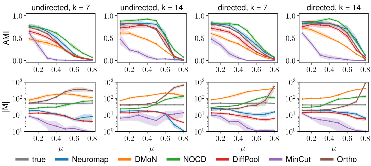
This figure presents the performance comparison of Neuromap (using different neural network architectures) and Infomap on directed and undirected LFR benchmark networks with planted communities. The performance is evaluated using three metrics: Adjusted Mutual Information (AMI) which measures the accuracy of the community detection, the number of detected communities (M), and the codelength (L) representing the description length of the random walk. The x-axis represents the mixing parameter (μ) which controls the level of mixing between communities, and different lines represent different methods. The shaded regions indicate standard deviation across multiple runs for each method and parameter.
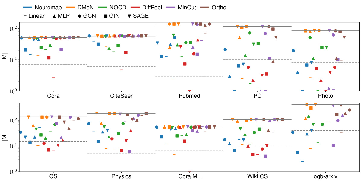
The figure shows the average achieved AMI (Adjusted Mutual Information) on ten real-world networks, comparing the performance of Neuromap against several baselines across different neural network architectures. The maximum number of communities (s) is set to the square root of the number of nodes (√n) for each dataset. The dashed horizontal lines indicate the ground truth number of communities. The plot also visualizes the impact of different neural network architectures on the performance.
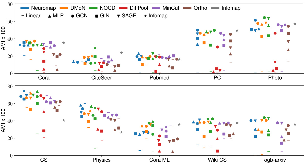
The figure shows the performance of different community detection methods on ten real-world datasets. The AMI (Adjusted Mutual Information) score, a measure of clustering quality, is plotted for each method and network architecture. The horizontal dashed lines represent the ground truth number of communities for each dataset. The plot highlights that Neuromap and several other methods achieve comparable or better performance than the baselines. One method (DiffPool) ran out of memory on the largest dataset, indicating a limitation in scalability.
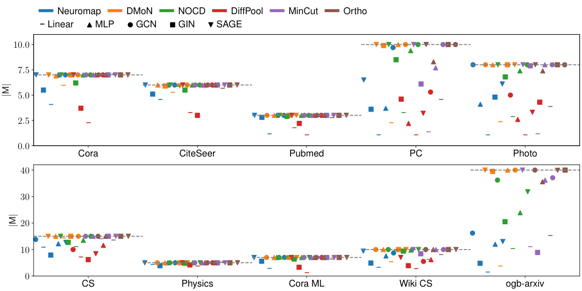
This figure shows the average achieved AMI (Adjusted Mutual Information) on ten real-world datasets for various community detection methods. The AMI score quantifies how well the detected communities match the ground truth. The different colors represent different community detection methods, and the different shapes represent the underlying neural network architecture used by each method. Note that the DiffPool method ran out of memory for the ogb-arxiv dataset. The horizontal lines indicate the maximum number of communities allowed for each dataset, reflecting the chosen maximum number of communities s=√n
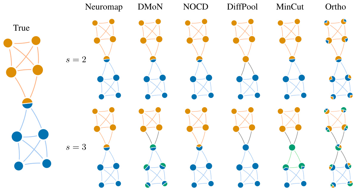
This figure shows the results of different community detection methods on a small synthetic network with overlapping communities. The network has nodes that belong to multiple communities simultaneously. The ‘True’ column displays the ground truth community structure. The remaining columns show the results of Neuromap and several baseline methods (DMON, NOCD, DiffPool, MinCut, Ortho) for allowing either a maximum of two or three communities, respectively. The visualization of nodes as pie charts helps understand the proportion of each node belonging to different communities, clearly demonstrating the performance of each method in detecting overlapping communities.
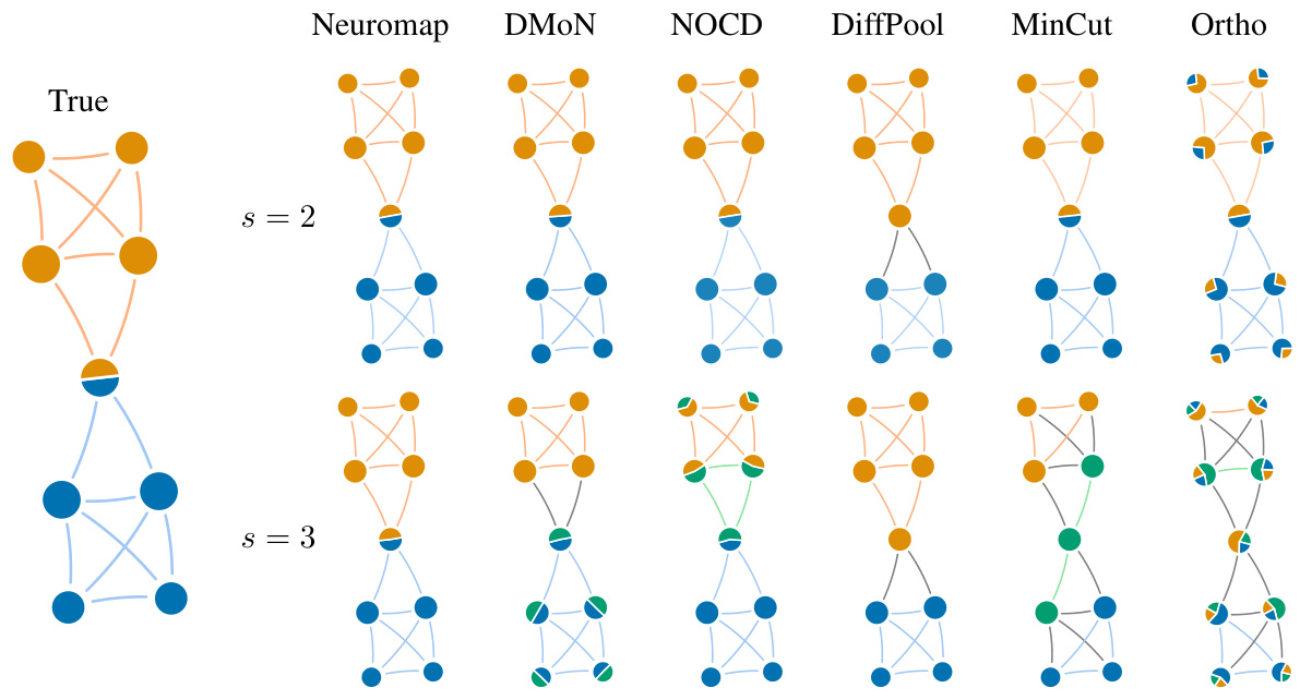
This figure compares different community detection methods on a small synthetic network with overlapping communities. The true community structure is shown on the leftmost side. Each subsequent column shows the community assignments detected by a different method: Neuromap, DMON, NOCD, DiffPool, MinCut, and Ortho. The top and bottom rows represent the results obtained when allowing a maximum of 2 or 3 communities, respectively. The visual representation of nodes as pie charts helps to illustrate the degree of community overlap detected by each method.
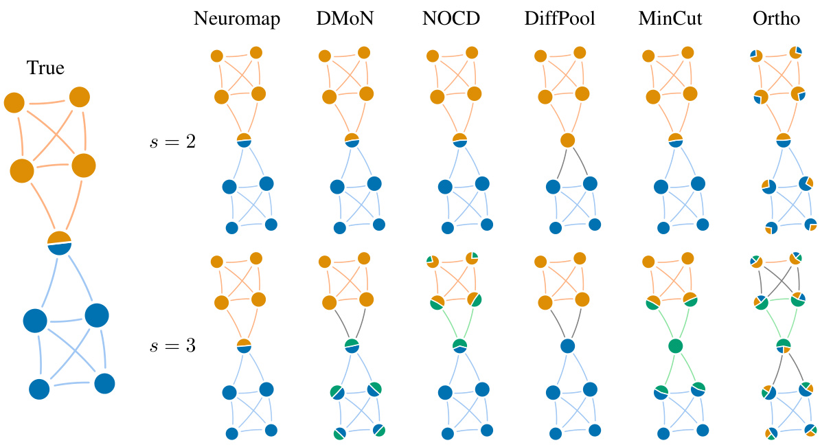
This figure compares the results of different community detection methods on a small synthetic network with overlapping communities. The true community structure is shown in the leftmost column. The remaining columns show the results obtained by Neuromap, DMON, NOCD, DiffPool, MinCut, and Ortho for a maximum number of communities (s) set to 2 and 3, respectively. The pie charts within each node represent the community assignment probabilities, visually illustrating the level of overlapping between communities.
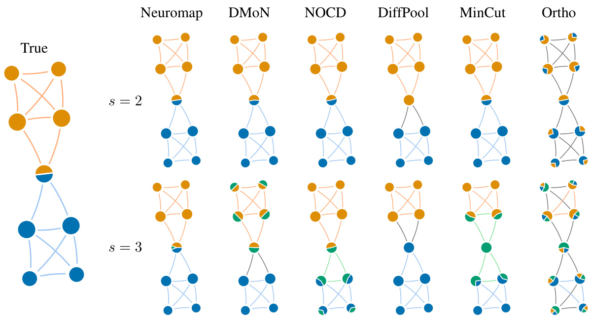
This figure presents a comparison of community detection methods on a small synthetic network with overlapping communities. The true community structure is shown in the leftmost column. The subsequent columns display the results of different community detection methods (Neuromap, DMON, NOCD, DiffPool, MinCut, Ortho), with each method’s results presented for a maximum of 2 and 3 communities, respectively. The visualization uses pie charts within each node to illustrate the proportion of the node’s membership in each community, thereby showcasing the ability (or lack thereof) of each method to identify and handle overlapping communities.
More on tables
This table presents the characteristics of ten real-world datasets used in the paper’s experiments. For each dataset, it lists the source, type (directed or undirected), number of nodes (|V|), number of edges (|E|), node feature dimension (|X|), number of communities (|Y|), and the mixing parameter (µ). The mixing parameter represents the proportion of inter-community edges, providing insights into the dataset’s community structure complexity.
This table lists properties of ten real-world datasets used in the paper’s experiments. For each dataset, it provides the source, type (directed or undirected), number of nodes (|V|), number of edges (|E|), node feature dimension (|X|), number of communities (|Y|), and the mixing parameter (µ). The mixing parameter quantifies how well the community structure is defined, with a lower value indicating a clearer community structure.
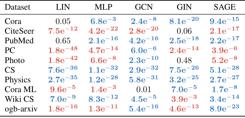
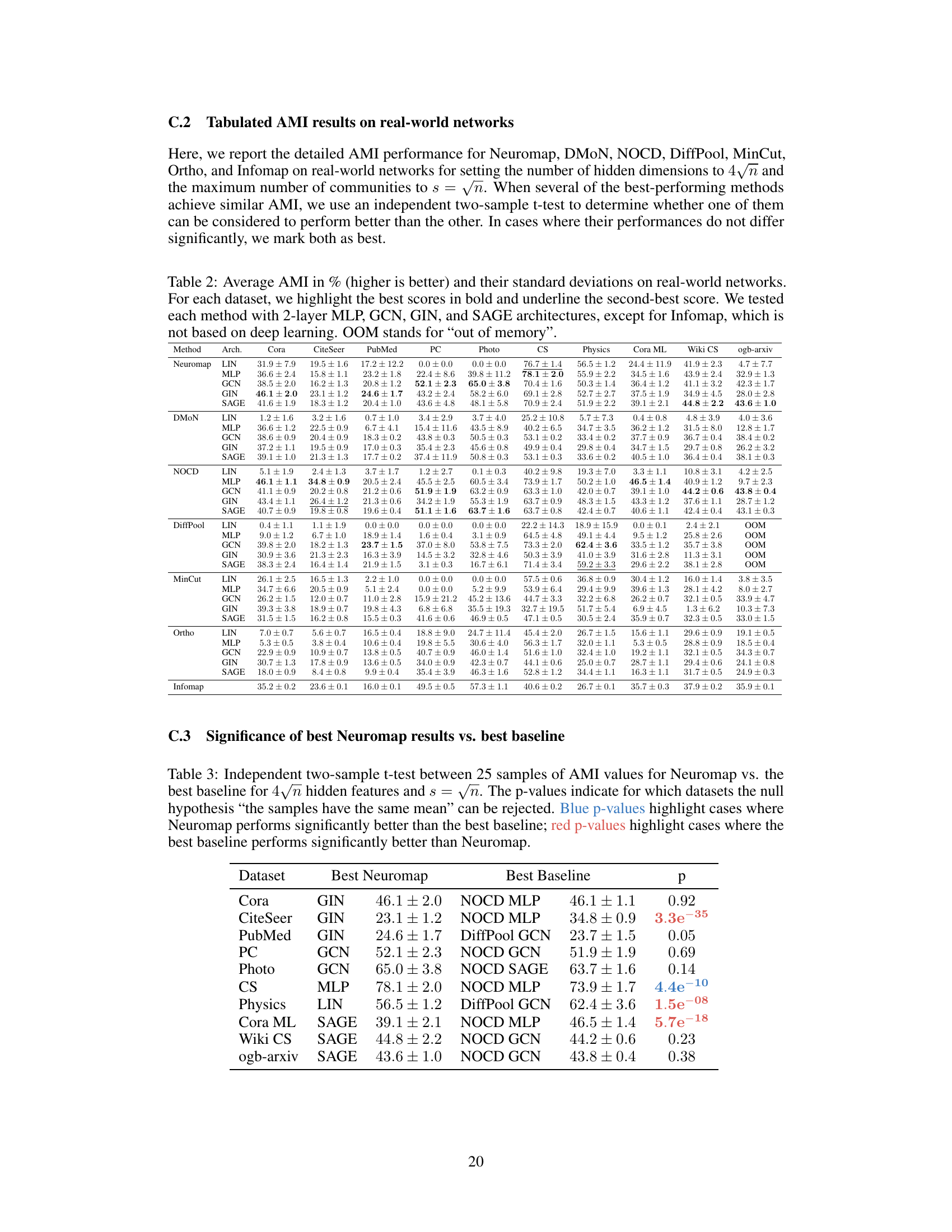
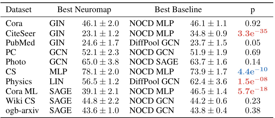
This table shows the results of independent two-sample t-tests comparing the performance of Neuromap against Infomap. The tests assess whether the mean AMI scores are significantly different for each method across various datasets. Blue p-values indicate statistically significant better performance for Neuromap, while red p-values show statistically significant better performance for Infomap. The different neural network architectures used (LIN, MLP, GCN, GIN, SAGE) are also listed, showing p-values for each.
This table presents the characteristics of ten real-world datasets used in the paper’s experiments. It lists the source of each dataset, whether it’s directed or undirected, the number of nodes (|V|), the number of edges (|E|), the node feature dimension (|X|), the number of communities (|Y|), and the mixing parameter (µ). The mixing parameter represents the ratio of inter-community edges to the total number of edges, indicating the extent of community overlap in the datasets.
This table presents the characteristics of ten real-world datasets used in the paper’s experiments. For each dataset, it lists the source, whether the network is directed or undirected, the number of nodes (|V|), the number of edges (|E|), the node feature dimension (|X|), the number of communities (|Y|), and the mixing parameter (μ). The mixing parameter indicates the level of overlap or randomness in the community structure.
This table presents the characteristics of ten real-world datasets used in the paper’s experiments. It lists the source of each dataset, whether it is directed or undirected, the number of nodes (|V|), the number of edges (|E|), the node feature dimension (|X|), the number of communities (|Y|), and the mixing parameter (µ). The mixing parameter reflects the extent to which nodes are connected to nodes outside their community.
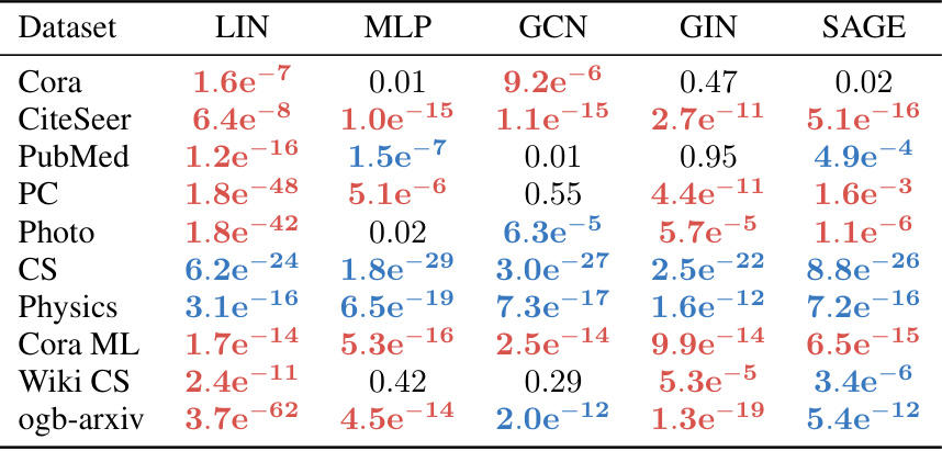
This table presents the results of independent two-sample t-tests comparing the performance of Neuromap (with various GNN architectures) against Infomap. The tests assess whether there’s a statistically significant difference in the average Adjusted Mutual Information (AMI) scores between the two methods. The p-values indicate the statistical significance of the difference; low p-values suggest a significant difference, favoring either Neuromap or Infomap, depending on the color-coding.
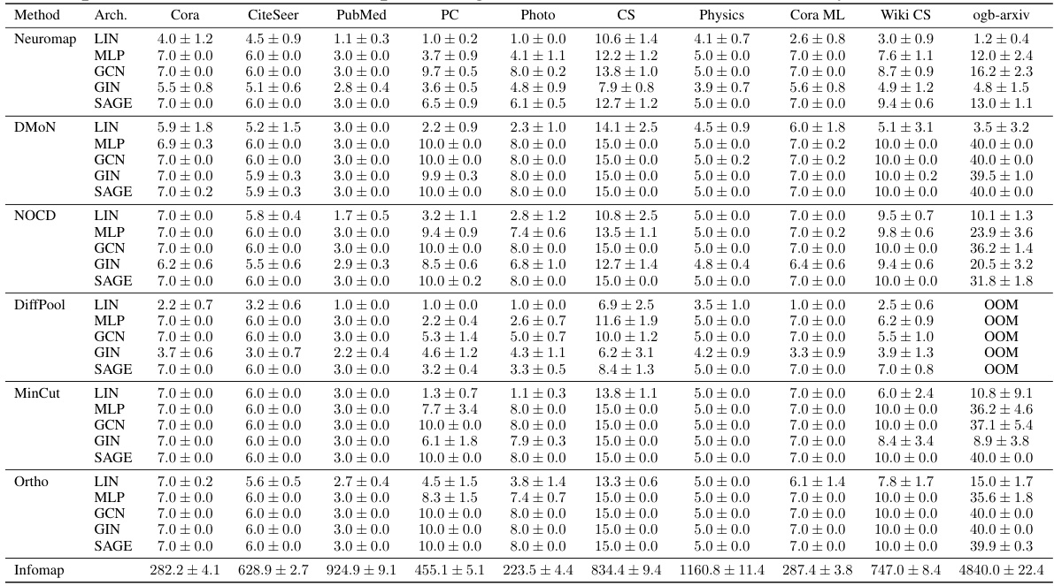
This table presents the characteristics of ten real-world datasets used in the paper’s experiments. Each dataset is described by its source, whether it is directed or undirected, the number of nodes (|V|), the number of edges (|E|), the dimensionality of node features (|X|), the number of ground-truth communities (|Y|), and the mixing parameter (µ). The mixing parameter represents the proportion of edges that connect nodes in different communities.
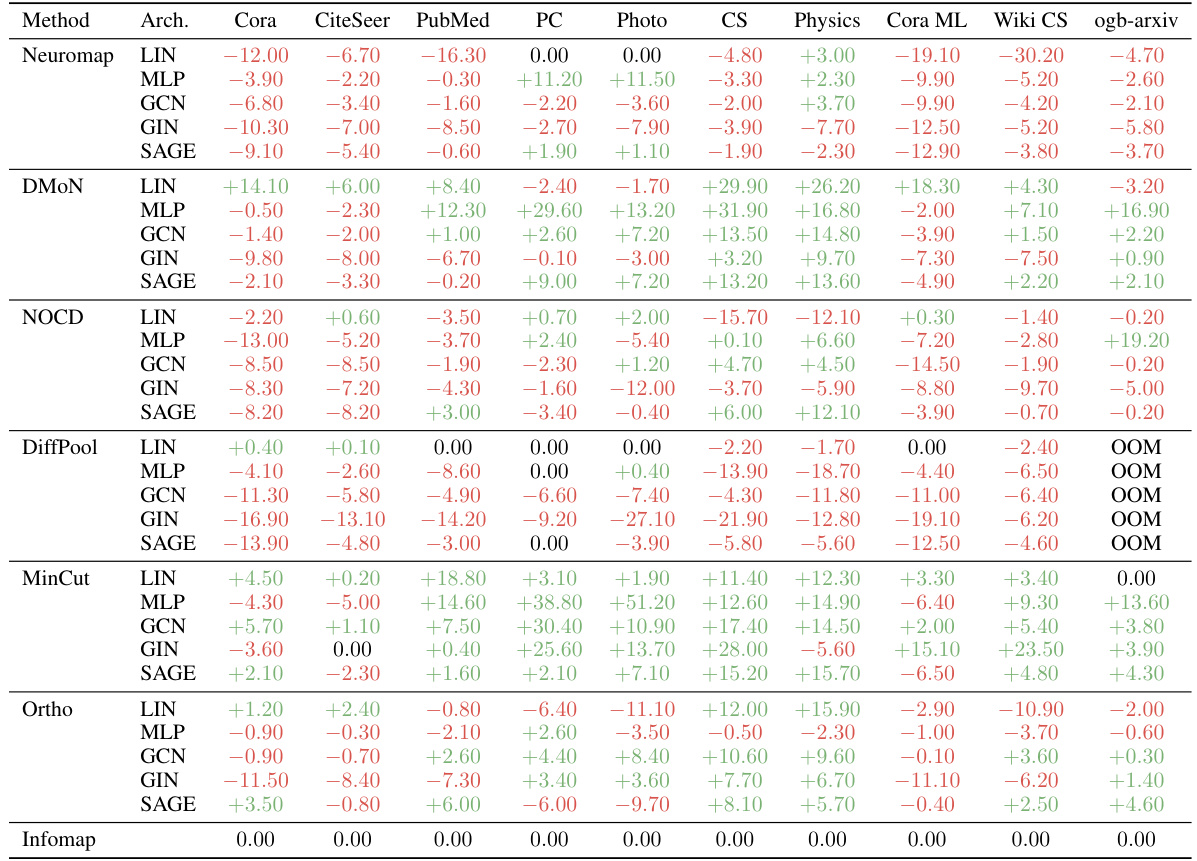
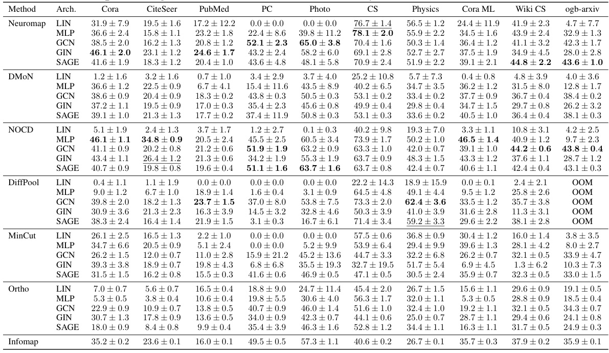
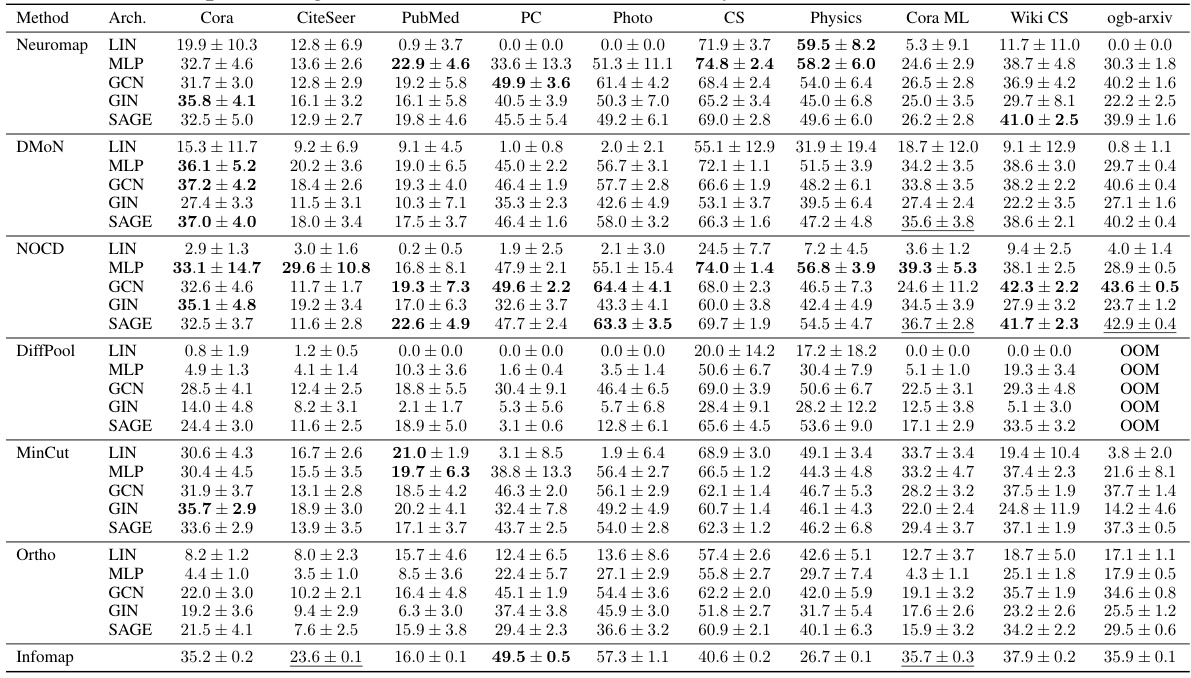
This table shows the average adjusted mutual information (AMI) achieved by different methods (Neuromap, DMON, NOCD, DiffPool, MinCut, Ortho, and Infomap) on ten real-world datasets. Different neural network architectures (MLP, GCN, GIN, SAGE) were used with Neuromap, while Infomap is not based on deep learning. The best AMI scores for each dataset are highlighted in bold and the second-best are underlined. The table also notes instances where methods ran out of memory (OOM).
Full paper#
