TL;DR#
Traditional statistical learning theory assumes a fixed data distribution, which is often unrealistic. Real-world data often exhibit variability, causing challenges in model generalization. This paper tackles these issues by introducing a new learning setting that explicitly models this variability.
This new approach, called Credal Learning Theory, uses convex sets of probabilities (credal sets) to represent the uncertainty in the data distribution. The paper derives generalization bounds under this credal uncertainty, offering more robust guarantees for model performance than traditional methods. The authors demonstrate how classical learning theory results are special cases of their new, more general results.
Key Takeaways#
Why does it matter?#
This paper is crucial for researchers grappling with data distribution shifts in machine learning. It provides novel theoretical frameworks and generalization bounds under credal uncertainty, addressing a significant challenge in real-world applications. The work opens new avenues for research by suggesting the use of imprecise probabilities, leading to more robust and reliable models.
Visual Insights#

🔼 This figure illustrates the process of credal learning. Multiple training datasets, each potentially generated from a different distribution, are used to infer a credal set (a convex set of probability distributions). This credal set represents the uncertainty in the data-generating process. From this credal set, generalization bounds can be derived under credal uncertainty which provides a more robust estimate of model risk compared to traditional methods that assume a single data generating distribution.
read the caption
Figure 1: Graphical representation of the proposed learning framework. Given an available finite sample of training sets, each assumed to be generated by a single data distribution, one can learn a credal set P of data distributions in either a frequentist or subjectivist fashion (Section 3). This allows us to derive generalization bounds under credal uncertainty (Section 4).

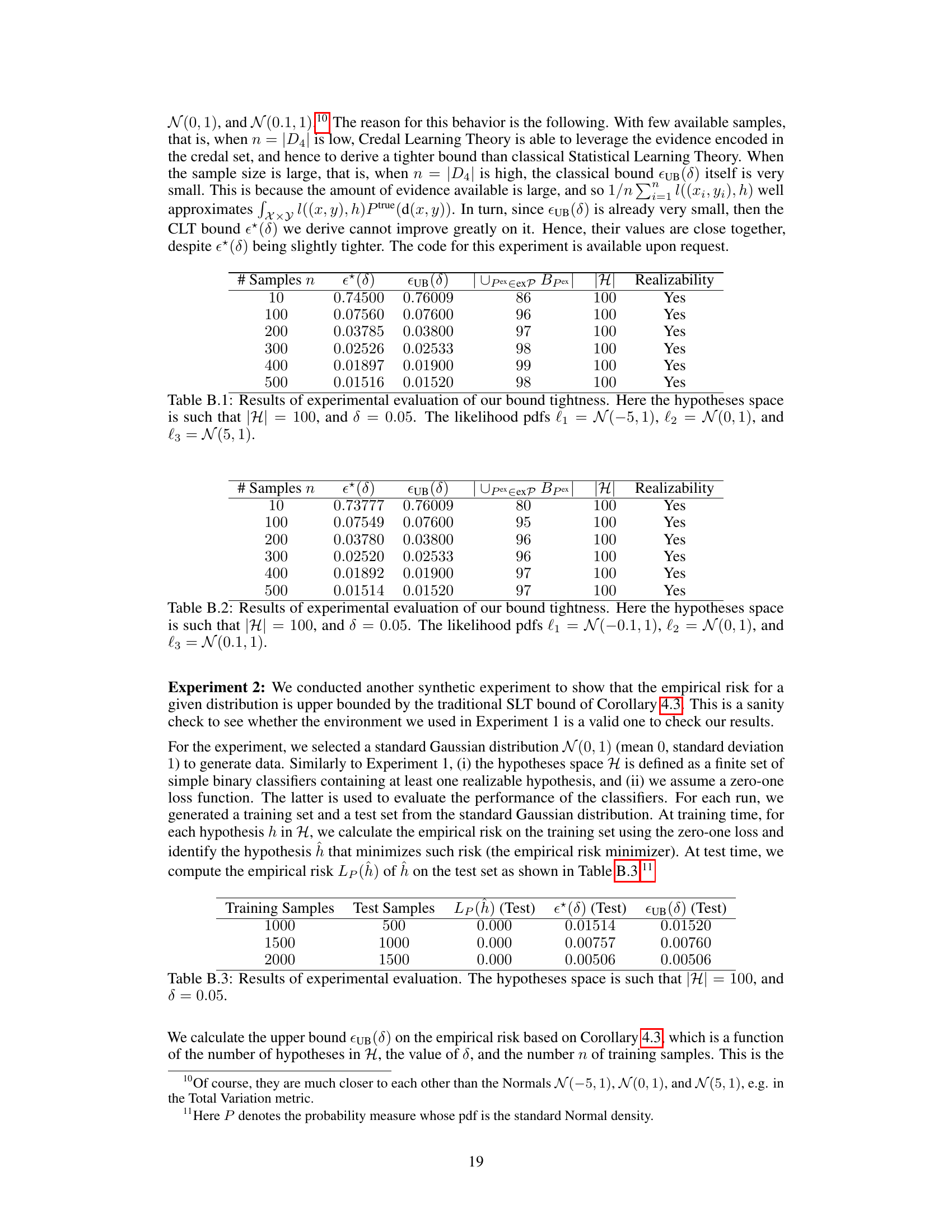
🔼 This table presents the results of an experiment evaluating the tightness of the bound derived in Theorem 4.1. It shows the empirical risk (ε*(δ)) and the classical SLT bound (εUB(δ)) for various sample sizes (n), along with the number of hypotheses in the set of ‘bad hypotheses’ (|Upex∈expBpex|) and the total number of hypotheses in the space (|H|). Realizability (whether a hypothesis exists with zero expected risk) is also indicated. The experiment uses three normal distributions with different means as likelihoods to construct a credal set.
read the caption
Table B.1: Results of experimental evaluation of our bound tightness. Here the hypotheses space is such that |H| = 100, and δ = 0.05. The likelihood pdfs l₁ = N(−5,1), l2 = N(0,1), and l3 = N(5, 1).
In-depth insights#
Credal Learning#
The concept of ‘Credal Learning’ introduces a novel approach to statistical learning theory by explicitly acknowledging and modeling the uncertainty inherent in real-world data distributions. Instead of assuming a single, unknown data-generating distribution, it leverages imprecise probabilities, specifically credal sets (convex sets of probability distributions), to represent the variability and uncertainty in the data. This framework is particularly relevant when dealing with situations of domain adaptation or generalization where the data distribution is likely to shift or be imprecisely known. By utilizing credal sets, ‘Credal Learning’ offers a more robust and flexible approach to deriving generalization bounds, providing more reliable uncertainty quantification in model predictions. A key strength lies in its ability to incorporate both frequentist and subjectivist modeling techniques, offering flexibility in how the credal set is constructed. The resulting generalization bounds derived under credal uncertainty are more robust and less sensitive to variations in the data generating process, generalizing classical SLT results as special cases. However, challenges related to computational complexity and practical elicitation of credal sets remain areas for further exploration.
Gen Bounds#
The heading ‘Gen Bounds’, likely short for ‘Generalization Bounds’, in a machine learning research paper signifies a critical section focused on theoretical guarantees of a model’s performance on unseen data. It would delve into mathematical expressions and inequalities that quantify the risk or error a model might incur when deployed beyond its training dataset. A strong emphasis will be placed on how model complexity, the size and nature of the training data, and properties of the hypothesis space relate to generalization capability. Different types of bounds (e.g., Rademacher complexity, VC-dimension) will likely be explored, each offering unique insights into the model’s expected error. The section will demonstrate how these bounds can be used to assess the reliability and generalizability of learned models, showing conditions under which high accuracy on training data translates into reliable performance on new, unseen data points. It serves as a cornerstone in justifying model selection and algorithm design.
Realizability#
The concept of ‘Realizability’ in machine learning, particularly within the context of statistical learning theory, is crucial. It essentially refers to the existence of a perfect model within the hypothesis space. This means there’s at least one model that can perfectly predict the output given the input, resulting in zero expected risk. A key implication of realizability is that it simplifies the analysis of generalization bounds. When realizability holds, we can derive tighter bounds on the model’s performance on unseen data. This is because the presence of a perfect model provides a benchmark against which the learned model can be compared. However, the realizability assumption is often unrealistic in practice. Real-world data is inherently noisy and complex, and it’s unlikely a perfect model exists. Therefore, theoretical results based on realizability often don’t translate directly to practical applications. Consequently, much research focuses on extending the theory to scenarios where realizability doesn’t hold, leading to more complex but applicable results. These generalizations typically involve incorporating measures of model complexity and the degree of data noise into the analysis. Relaxing the realizability assumption is essential for bridging the gap between theoretical results and practical applications of machine learning models.
Infinite Spaces#
When dealing with infinite hypothesis spaces in machine learning, the challenge of generalization intensifies significantly. Classical statistical learning theory often struggles to provide meaningful bounds on the expected risk of models learned from finite data sets. This is because the sheer number of potential hypotheses is unbounded, increasing the probability of overfitting. The introduction of credal learning theory offers a potential solution, leveraging sets of probability distributions (credal sets) to account for uncertainty in the data generation process. By considering a range of possibilities instead of a single point estimate, credal learning allows for robust generalization bounds even in high-dimensional infinite spaces. This approach moves beyond the limitations of traditional methods which typically rely on strong assumptions, such as realizability or boundedness, that are often unrealistic in practice. Therefore, credal learning provides a more nuanced and practical framework for tackling the complex theoretical and computational challenges of learning within infinite hypothesis spaces. The use of credal sets requires careful consideration of computational costs but potentially yields stronger and more reliable results compared to classical methods.
Future Work#
The paper’s “Future Work” section hints at several promising directions. Extending the framework to handle losses beyond zero-one loss is crucial for broader applicability. Addressing the computational complexity of credal sets, especially for larger datasets, is vital for practical implementation. The investigation of PAC-like guarantees on the correct distribution being within the credal set is a theoretical cornerstone needing further exploration. Finally, the authors plan empirical validation on real-world datasets, a necessary step to demonstrate the practical benefits of the proposed credal learning theory in diverse applications. The integration of incremental learning to continually refine the credal set also holds potential.
More visual insights#
More on figures

🔼 This figure illustrates the overall framework of the proposed credal learning approach. It shows how a finite sample of training sets, each from a potentially different distribution, is used to infer a credal set (a convex set of probability distributions) representing the uncertainty in the data-generating process. This credal set then forms the basis for deriving generalization bounds, providing robust uncertainty quantification.
read the caption
Figure 1: Graphical representation of the proposed learning framework. Given an available finite sample of training sets, each assumed to be generated by a single data distribution, one can learn a credal set P of data distributions in either a frequentist or subjectivist fashion (Section 3). This allows us to derive generalization bounds under credal uncertainty (Section 4).
🔼 The figure shows a graphical model of the proposed learning framework. It begins with a finite sample of training sets, each assumed to be generated by a single unknown data distribution. From these, a credal set (convex set) of probability distributions is inferred using either frequentist or subjectivist methods. This credal set is then used to derive generalization bounds under credal uncertainty, which are bounds on the expected risk given the uncertainty represented by the credal set. This framework allows for more robust generalization bounds by acknowledging variability in the data-generating distribution.
read the caption
Figure 2. Graphical representation of the proposed learning framework. Given an available finite sample of training sets, each assumed to be generated by a single data distribution, one can learn a credal set P of data distributions in either a frequentist or subjectivist fashion (Section 3). This allows us to derive generalization bounds under credal uncertainty (Section 4).
More on tables

🔼 This table presents the results of an experiment designed to evaluate the tightness of the bound derived in the paper. It shows how the bound (ε*(δ)) compares to a classical bound (εUB(δ)) for various sample sizes (n). The experiment used a hypothesis space (H) of size 100 and a significance level (δ) of 0.05. The likelihoods used were three normal distributions with means close to zero.
read the caption
Table B.2: Results of experimental evaluation of our bound tightness. Here the hypotheses space is such that |H| = 100, and δ = 0.05. The likelihood pdfs l₁ = N(−0.1,1), l2 = N(0, 1), and l3 = N(0.1, 1).

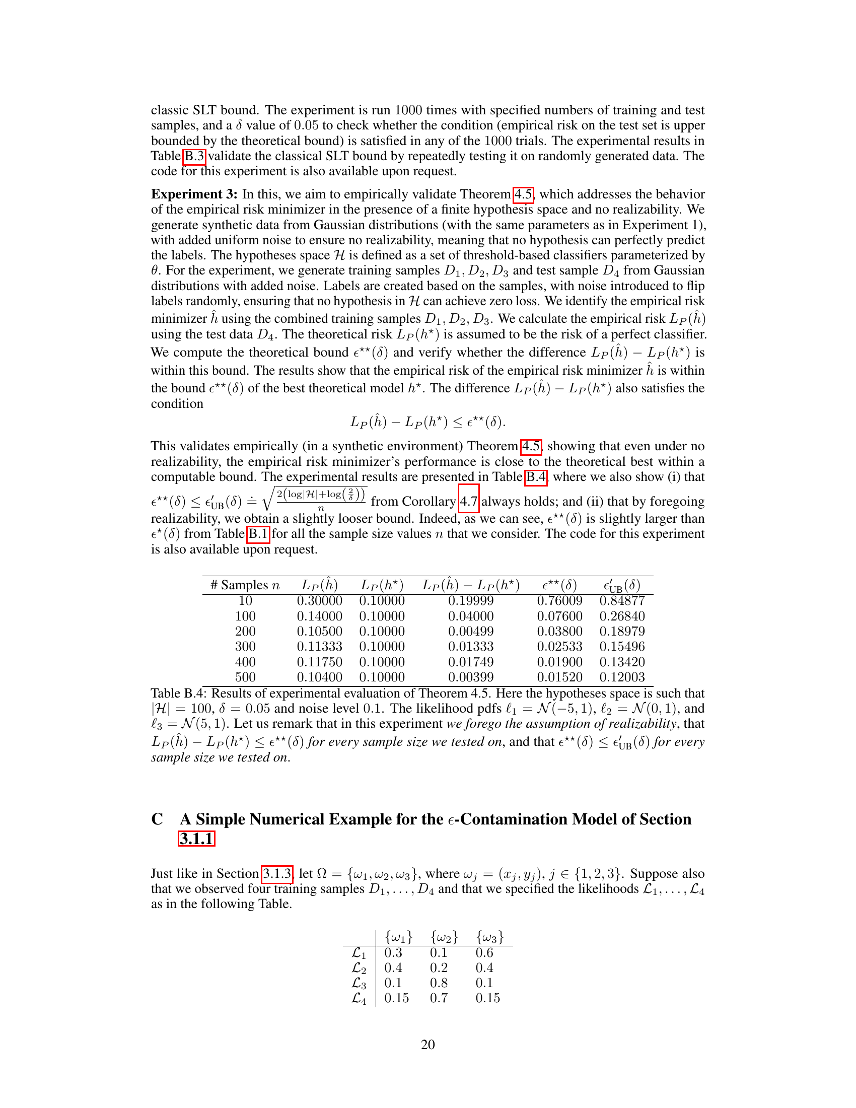
🔼 This table presents the results of an experimental evaluation to validate the classical SLT bound. It shows the empirical risk (Lp(h)) of the empirical risk minimizer (h) on test sets of different sizes (500, 1000, 1500), given training sets of varying sizes (1000, 1500, 2000). The classical SLT bound (εUB(δ)) and a tighter bound (ε*(δ)) from the paper are also displayed for comparison. The results demonstrate that the empirical risk is always below both theoretical bounds, confirming the validity of the classical SLT bound and showing the tighter bound from the paper.
read the caption
Table B.3: Results of experimental evaluation. The hypotheses space is such that |H| = 100, and δ = 0.05.

🔼 This table presents the results of an experiment designed to validate Theorem 4.5 of the paper. The theorem discusses the behavior of the empirical risk minimizer when there is no realizability (i.e., no hypothesis perfectly predicts the labels). The experiment uses synthetic data generated from Gaussian distributions with added noise to simulate non-realizability. The table shows, for different sample sizes, the empirical risk of the learned model (Lp(ĥ)), the risk of the best theoretical model (Lp(h*)), the difference between these two risks, and the theoretical bounds from Theorem 4.5 (ε**(δ)) and Corollary 4.7 (ε’UB(δ)). The results show that the difference in risk between the empirical minimizer and the theoretical optimum is consistently within the bounds predicted by the theorem, even in the absence of realizability.
read the caption
Table B.4: Results of experimental evaluation of Theorem 4.5. Here the hypotheses space is such that |H| = 100, δ = 0.05 and noise level 0.1. The likelihood pdfs l₁ = N(−5,1), l2 = N(0,1), and l3 = N(5, 1).

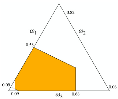
🔼 This table presents the lower and upper probabilities derived from the credal set P, which is obtained from the example in Section 3.1.3 where belief functions are inferred from data. The table shows the lower and upper probability values for various subsets of the sample space Ω = {ω₁, ω₂, ω₃}, illustrating the range of possible probability assignments consistent with the available evidence. This exemplifies the concept of imprecise probabilities, where uncertainty is represented by a set of probabilities rather than a single point estimate.
read the caption
Table 2. Table 2.
Full paper#

