↗ OpenReview ↗ NeurIPS Homepage ↗ Hugging Face ↗ Chat
TL;DR#
Many deep learning models exist for approximating solutions to partial differential equations (PDEs), but they often face limitations in handling complex geometries and long-term predictions. Neural operators, while powerful, are often constrained by discretization and domain geometry. Neural fields, while flexible, struggle with modeling spatial information and local dynamics effectively; existing transformer architectures are computationally expensive. This research addresses these challenges.
The paper introduces AROMA, a novel framework that leverages attention blocks and neural fields for PDE modeling. AROMA uses a flexible encoder-decoder architecture to create smooth latent representations of spatial fields from various data types, eliminating the need for patching. Its sequential latent representation allows for spatial interpretation, enabling the use of a conditional transformer to model temporal dynamics. A diffusion-based formulation enhances stability and allows for longer-term predictions. Experimental results demonstrate AROMA’s superior performance compared to conventional methods.
Key Takeaways#
Why does it matter?#
This paper is important because it presents AROMA, a novel framework that significantly improves the modeling of partial differential equations (PDEs), particularly for complex geometries. Its efficiency in handling diverse geometries and data types, along with its superior performance compared to existing methods, makes it highly relevant to various scientific and engineering domains. The diffusion-based approach enhances stability and allows for longer-term predictions, opening new avenues for research in spatio-temporal modeling.
Visual Insights#
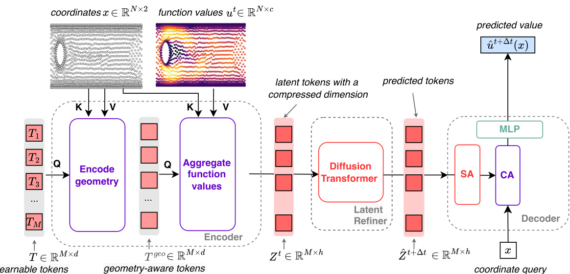
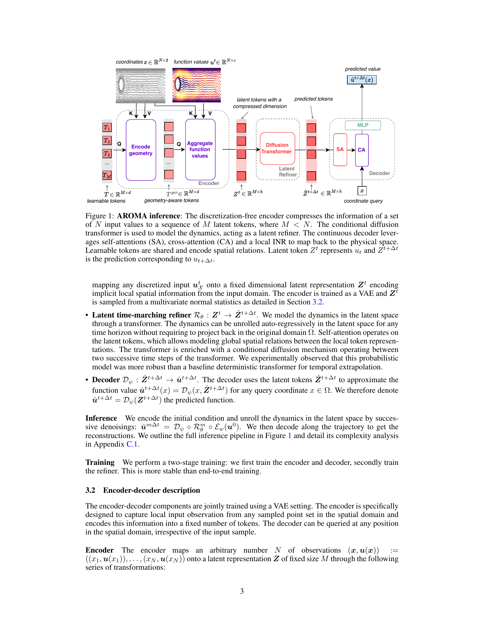
This figure illustrates the AROMA model’s inference process. The input, representing spatial data (e.g., from a grid, mesh, or point cloud), is first encoded into a compressed latent representation using a discretization-free encoder. This latent representation, consisting of M tokens (M « N, where N is the number of input values), is then processed by a conditional diffusion transformer to model the temporal dynamics of the system. Finally, a decoder maps the refined latent tokens back into the original physical space to provide the prediction at any desired location.

This table compares the performance of AROMA against various state-of-the-art baselines on three different datasets: Burgers, Navier-Stokes 1e-4, and Navier-Stokes 1e-5. The performance is measured using the Relative L2 error metric. The results highlight AROMA’s superior performance in capturing the dynamics of turbulent phenomena, especially compared to global neural field methods like DINO and CORAL, which struggle with turbulent data. AROMA also shows competitive results against other regular-grid methods like FNO and GNOT.
In-depth insights#
Latent Space Dynamics#
Analyzing latent space dynamics in the context of a research paper unveils how the model’s internal representation evolves over time. This is crucial for understanding the model’s learning process and how it captures the underlying dynamics of the system being modeled. By visualizing the trajectories of latent tokens, we can observe the flow and interactions within the reduced-dimensional space, and relate them to the model’s predictions. The presence of noise or uncertainty in the latent space can also be quantified and linked to the confidence of model predictions. Investigating these patterns allows researchers to identify areas of stability, instability, and the ability of the latent space to accurately model the original system’s complexity. Furthermore, a detailed analysis can reveal whether the latent space fully captures the essence of the original data, or whether crucial information is lost during the dimensionality reduction process. This analysis is critical for assessing the model’s ability to generalize and make accurate predictions beyond the training data.
Geometry Encoding#
Geometry encoding in the context of PDE modeling using neural fields is a crucial step that significantly impacts the model’s ability to handle diverse spatial domains. The core idea is to translate the complex geometric information of a given domain (e.g., irregular meshes, point clouds) into a compact and efficient representation that can be readily processed by neural networks. This encoding process allows the model to generalize well to unseen geometries and overcome the limitations of traditional methods constrained by specific grid structures. Effective geometry encoding leads to a discretization-free approach, enhancing the model’s flexibility and versatility. Different strategies could involve using positional embeddings, graph neural networks, or other techniques to capture local and global spatial relationships within the domain. The choice of encoding method directly affects the model’s computational efficiency and its capacity to capture the intricacies of the underlying physical phenomena. An effective geometry encoding scheme should balance compactness with the preservation of crucial spatial information. This balance is critical for achieving accurate and efficient PDE solutions, particularly in scenarios with complex geometries or sparse data.
Diffusion Refinement#
Diffusion refinement, in the context of latent space modeling for partial differential equations, offers a powerful technique to enhance the stability and accuracy of long-term predictions. By incorporating a diffusion process within the latent space, the model can effectively handle the accumulation of errors inherent in autoregressive forecasting. This approach differs significantly from deterministic methods, which tend to suffer from instability as the prediction horizon increases. The probabilistic nature of the diffusion process allows the model to account for uncertainty in the latent dynamics, leading to more robust and reliable predictions even when dealing with complex, chaotic systems. Furthermore, the diffusion process can be seamlessly integrated with other components of the latent space modeling pipeline. For example, it can be combined with attention mechanisms to effectively capture spatial and temporal dependencies, thus offering a significant improvement in performance compared to conventional techniques such as MSE training. The use of a diffusion-based refinement step represents a novel and effective way to address the challenges of long-term forecasting and enhances the overall reliability of the PDE modeling framework.
Ablation Studies#
Ablation studies systematically remove components of a model to assess their individual contributions. In this context, it’s likely the authors tested variations of their model, such as removing the diffusion process, altering the number of latent tokens, or modifying the architecture of the encoder-decoder. The results would show the impact of each component on key metrics like reconstruction error and predictive accuracy. A key takeaway would be identifying the most critical components for the model’s overall performance. The analysis would help determine which aspects are most essential and which could be potentially simplified or improved without significant performance loss. This is critical for understanding model behavior and optimizing its efficiency. The ablation study provides valuable insight into the model’s strengths and weaknesses, enabling the researchers to refine their approach and potentially create a more streamlined version, which is important for reproducibility and resource-efficient deployment.
Future Work#
Future research directions stemming from this work could explore several promising avenues. Extending AROMA to handle more complex PDEs and higher-dimensional systems would significantly broaden its applicability. Investigating the impact of different attention mechanisms and exploring alternative latent space representations could lead to improvements in accuracy and efficiency. A thorough analysis of uncertainty quantification within AROMA’s framework is critical, particularly for long-term predictions. This could involve developing more robust probabilistic models or integrating techniques from Bayesian deep learning. Incorporating adaptive mesh refinement strategies into the architecture would enhance its ability to resolve fine-scale details in complex geometries. Finally, exploring the use of AROMA in other scientific domains beyond fluid dynamics and evaluating its performance on real-world datasets should be prioritized.
More visual insights#
More on figures

The figure illustrates the AROMA model’s inference process. It starts with input values, which are encoded into a compressed latent representation using a discretization-free encoder. This latent representation then undergoes a time-marching process using a conditional diffusion transformer, which refines the latent tokens over time. Finally, a decoder maps these refined tokens back to the original space, providing predictions. Self-attention and cross-attention mechanisms are used within the transformer for modeling relationships between latent tokens, while a local INR enables continuous mapping back to the original space.
This figure illustrates the AROMA model’s inference process. The input data (N values) is first encoded into a smaller, fixed-size latent representation (M tokens, M<N) that captures spatial information efficiently. This compact latent representation is then processed by a diffusion transformer to model the temporal dynamics. Finally, a decoder maps the refined latent representation back to the original spatial domain, allowing for predictions at any location.

This figure compares the performance of different models (FNO, ResNet, AROMA, and AROMA without diffusion) on long-term prediction tasks. The x-axis represents the number of rollout steps (time), while the y-axis shows the correlation between the model predictions and the ground truth. The plot reveals how the correlation decreases over time for all models, indicating that the predictive accuracy degrades as the prediction horizon extends. AROMA with diffusion outperforms the other methods in maintaining a higher correlation for a longer period.

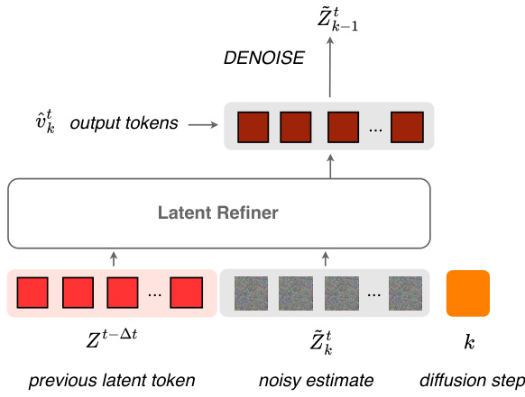
This figure illustrates the training process of the diffusion transformer block within AROMA. The input consists of previous latent tokens (Zt-△t) and a noisy estimate of the current latent tokens (Zt). A linear layer maps the noisy estimate and the previous latent tokens to a higher dimensional space. Then a Diffusion Transformer (DiT) block, detailed in Appendix B, processes this information and outputs new tokens. These output tokens are compared to the target tokens using Mean Squared Error (MSE) to calculate the loss. A linear layer, as well as noise scheduling function (√αkϵ - √1-αk Zt), maps the diffusion step conditioning embedding (k) to the target tokens.
This figure illustrates the AROMA (Attentive Reduced Order Model with Attention) model architecture for solving Partial Differential Equations (PDEs). The process begins with an encoder that compresses input data (from various sources, such as point clouds or irregular grids) into a compact representation of latent tokens. A diffusion-based transformer then models the temporal dynamics within this lower-dimensional latent space. Finally, a decoder reconstructs the solution in the original space using a continuous neural field, generating values at any spatial location requested.
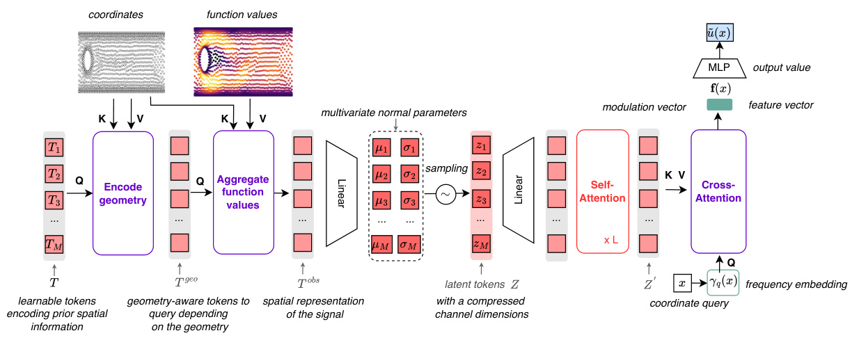
The figure illustrates the architecture of the AROMA model for solving PDEs. It shows how the input data is encoded into a lower-dimensional latent space, processed using a diffusion transformer to model the temporal dynamics, and then decoded back into the original space to obtain predictions. The encoder handles diverse geometries without discretization. The transformer refines the latent representation sequentially, and the decoder uses self-attention, cross-attention, and a local INR for accurate prediction.

This figure illustrates the inference process of the AROMA model for solving partial differential equations. The encoder takes in a set of N input values, which are then compressed into a smaller sequence of M latent tokens (where M < N). This compressed representation is then fed into a diffusion transformer which models the dynamics of the system over time. The output of the transformer, a refined set of latent tokens, is then passed to a decoder which uses self-attention, cross-attention, and a local implicit neural representation (INR) to reconstruct the continuous physical values, achieving a discretization-free approach. The figure highlights the model’s ability to handle both spatial and temporal information efficiently.
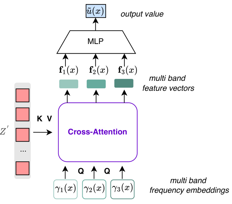
The figure shows the architecture of a multi-band local INR decoder. The decoder uses cross-attention to retrieve multiple feature vectors, each corresponding to a different frequency band. These feature vectors are then concatenated and passed through an MLP to produce the final output value. This multi-band approach allows the decoder to capture more detailed spatial information than a single-band decoder.

This figure illustrates the architecture of the AROMA model, which consists of three main components: an encoder, a latent time-marching refiner (diffusion transformer), and a decoder. The encoder takes the input values (e.g., spatial data) and converts them into a sequence of M latent tokens. The diffusion transformer processes these latent tokens to model the temporal dynamics of the system, making predictions in the latent space. Finally, the decoder maps the latent tokens back to the physical space to generate the output, such as prediction of spatiotemporal data.

This figure illustrates the AROMA model’s inference process. It begins with an encoder that takes input values (discretized or not) and compresses them into a smaller set of latent tokens, capturing essential spatial information. These tokens are then processed by a conditional diffusion transformer to model the temporal dynamics of the system. Finally, a decoder maps the refined latent tokens back to the physical space, generating predictions. The model uses self-attention and cross-attention mechanisms for efficient processing.

This figure illustrates the architecture of the AROMA model, showing how input values are encoded into a compact latent representation, processed by a diffusion transformer to model temporal dynamics, and decoded back into the physical space. The encoder compresses spatial information into a smaller number of tokens, while the decoder uses self-attention and cross-attention mechanisms to reconstruct the output. The conditional diffusion transformer allows for robust and efficient modeling of temporal dynamics.

This figure illustrates the overall architecture of the AROMA model for solving partial differential equations (PDEs). It shows how the model processes the input data using a three-stage pipeline: encoding, processing (using a conditional diffusion transformer), and decoding. The encoder maps the input data onto a fixed-size compact latent representation, which is then processed by the transformer to model the dynamics. Finally, the decoder maps this latent representation back into the physical space to obtain the predicted values.

This figure illustrates the AROMA model’s inference process. The encoder processes input data (spatial coordinates and function values) to generate a compressed latent representation. A transformer refines this representation to model the dynamics. Finally, a decoder maps the refined representation back to the original space, generating predictions for future time steps. Key elements include attention mechanisms and a local implicit neural representation (INR) for spatial processing.

This figure shows the architecture of the AROMA model, highlighting its three main components: the encoder, the latent time-marching refiner, and the decoder. The encoder processes the input data (spatial field values) and transforms it into a lower-dimensional latent representation. The refiner models the temporal dynamics in this latent space, enabling efficient forecasting. Finally, the decoder maps the refined latent representation back to the original high-dimensional space to predict the spatial field at future timesteps.

This figure illustrates the AROMA model’s inference process. The encoder takes in input values and compresses them into a smaller set of latent tokens. A transformer processes these tokens to model the temporal dynamics, acting as a refiner. Finally, a decoder maps the refined tokens back to the original physical space, using self-attention, cross-attention and a local implicit neural representation (INR).

This figure shows the architecture of the AROMA model. The encoder takes input values (e.g., from a point cloud or mesh) and compresses them into a lower-dimensional latent representation using attention mechanisms. This latent representation is then processed by a diffusion transformer to model temporal dynamics. Finally, the decoder reconstructs the output values from the latent representation. The figure highlights the key components: encoding, latent refinement, and decoding, all working together to approximate solutions to PDEs.

This figure shows the architecture of the AROMA model for solving PDEs. The encoder compresses input data into a lower-dimensional latent representation using attention mechanisms. A diffusion transformer processes this latent representation to model temporal dynamics. Finally, a decoder reconstructs the solution in the original spatial domain using a continuous neural field.

This figure shows the architecture of the AROMA model. The encoder takes in input values and maps them to a sequence of M latent tokens (M<N, where N is the number of input values). The conditional diffusion transformer then processes this sequence to model the dynamics, which is then decoded to approximate the function value for any query coordinate in the spatial domain. The model is discretization-free, meaning it can handle various input types such as point clouds and irregular grids.

This figure illustrates the AROMA model’s inference process. The encoder takes input values and compresses them into a smaller set of latent tokens. These tokens are then processed by a diffusion transformer to model the temporal dynamics, and finally decoded to approximate the function values at any spatial location. Self-attention and cross-attention mechanisms are used to model spatial relations.

This figure shows a schematic of the AROMA model’s inference process. The input data (ux) is processed by an encoder to create a compressed representation in a latent space (Zt). This latent representation is then processed by a diffusion transformer to model temporal dynamics, resulting in a refined latent representation (Zt+∆t). Finally, a decoder maps this refined latent representation back to the original physical space to produce the prediction (ût+∆t). The figure highlights the key components of the model and their interaction.

This figure illustrates the AROMA model’s inference process. The encoder takes in input values (e.g., from a grid or point cloud) and compresses them into a smaller set of latent tokens. These tokens are then processed by a diffusion transformer that models temporal dynamics. Finally, the decoder reconstructs the function values at any queried point in space using self-attention, cross-attention, and a local neural implicit representation (INR).

This figure illustrates the architecture of the AROMA model. The encoder maps the input data to a compact latent representation. The latent refiner processes this representation using a diffusion transformer to capture the temporal dynamics. The decoder finally maps this refined representation back into the original space using a local neural network, resulting in the prediction for the next time step. The whole process is continuous, eliminating the need for discrete spatial discretization.

The figure illustrates the AROMA model’s inference process. An encoder transforms input data (e.g., from a grid or point cloud) into a compact latent representation using a sequence of M tokens. A conditional diffusion transformer processes these tokens to model the temporal dynamics of the system. Finally, a decoder maps the refined latent tokens back to the original spatial domain, generating a prediction.
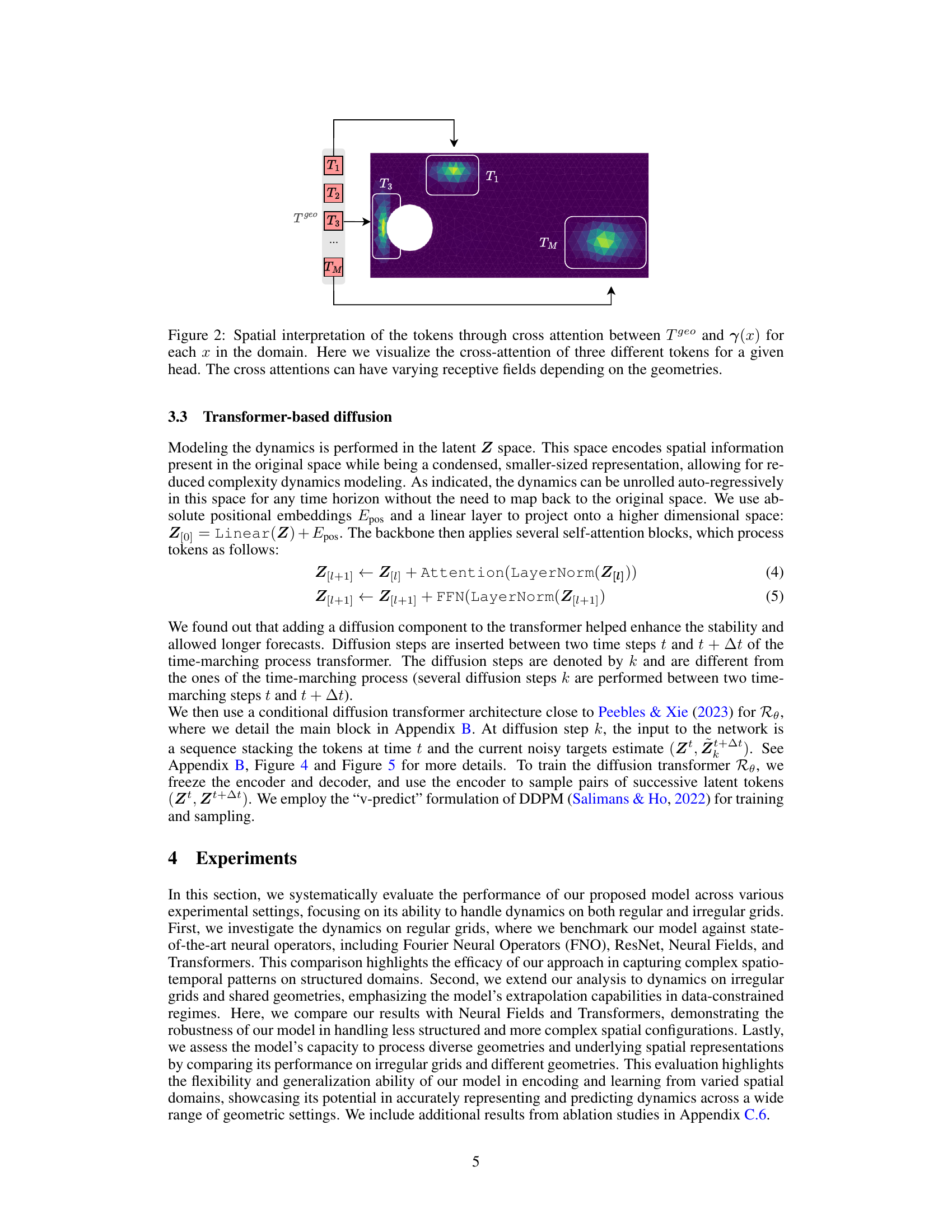
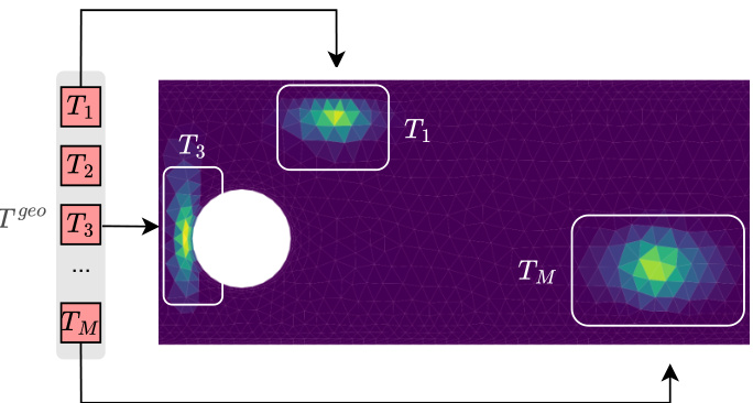
This figure shows how the model encodes spatial information through cross-attention. The heatmaps visualize the attention weights between geometry-aware tokens (Tgeo) and positional embeddings (γ(x)) for three different tokens. Varying receptive fields are observed, showing how the model adapts to different geometries. The spatial relationships are implicitly encoded in the latent token space.
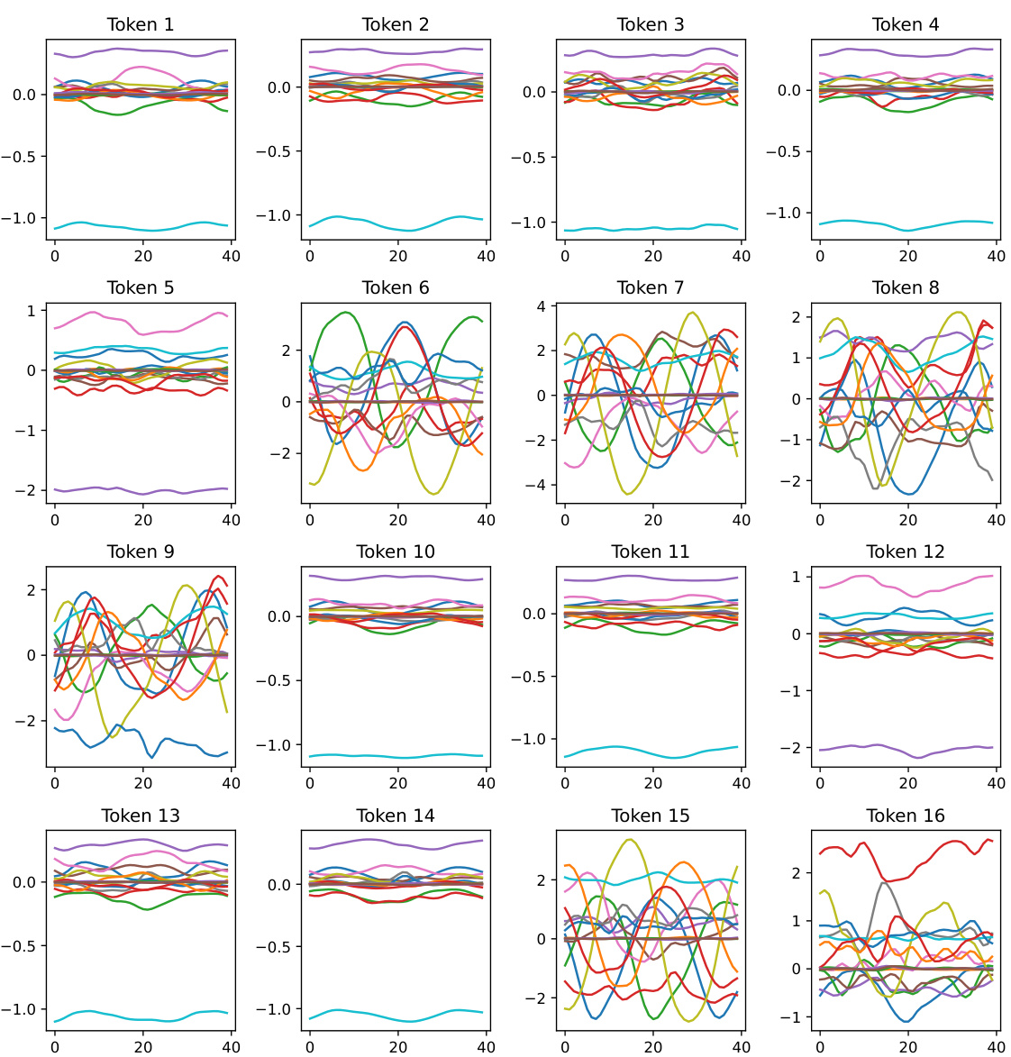
This figure illustrates the architecture of the AROMA model, which consists of three main components: an encoder, a diffusion transformer (latent time-marching refiner), and a decoder. The encoder compresses the input data (from various geometries) into a compact latent representation, which is then processed by the diffusion transformer to model temporal dynamics. Finally, the decoder maps the processed latent representation back into the original space, providing predictions for any query location.

The figure illustrates the AROMA model’s architecture, highlighting its three main components: the encoder, the latent time-marching refiner, and the decoder. The encoder transforms input values into a lower-dimensional latent space, capturing essential spatial information. A conditional diffusion transformer processes these latent tokens to model the temporal dynamics, while a continuous decoder maps back to the original physical space to provide predictions. The model’s key advantage is its ability to handle various data types and complex geometries, providing a flexible and efficient approach to PDE modeling.
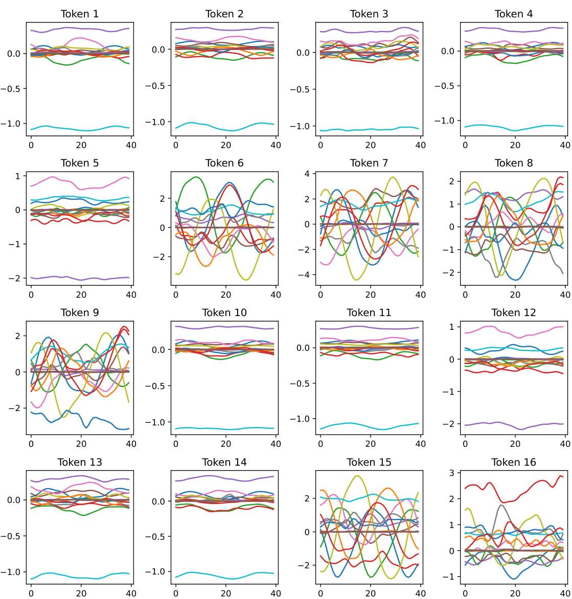
This figure illustrates the AROMA model’s inference process. The encoder takes input values and compresses them into a smaller set of latent tokens. A transformer processes these tokens to model temporal dynamics, refining the latent representation. Finally, a decoder maps the refined tokens back to the original space, providing a prediction of the function values.
More on tables
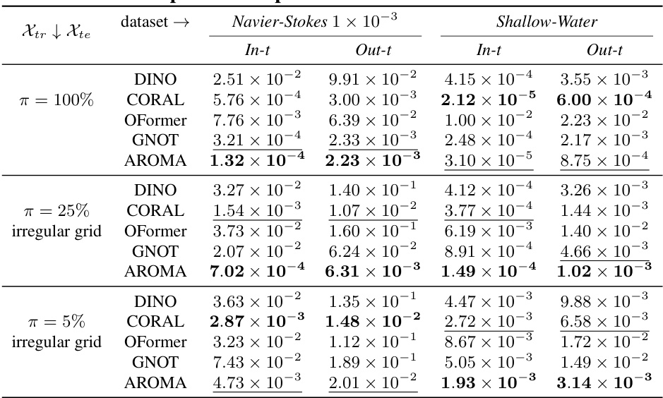
This table presents a comparison of the model’s performance on two datasets (Navier-Stokes 1 × 10⁻³ and Shallow-Water) across various levels of observation sparsity (π = 100%, 25%, 5%). The metrics reported are Mean Squared Errors (MSE) for both the training horizon (In-t) and extrapolation horizon (Out-t). The results highlight AROMA’s consistent performance across different sparsity levels and time horizons.

This table compares the performance of different models (CORAL, DINO, OFormer, and AROMA) on two fluid dynamics problems involving non-convex domains: CylinderFlow and AirfoilFlow. The results are presented as Mean Squared Error (MSE) on normalized data, for both the in-training horizon (‘In-t’) and the extrapolation horizon (‘Out-t’). The metrics evaluate the models’ ability to predict flow dynamics on different geometries.

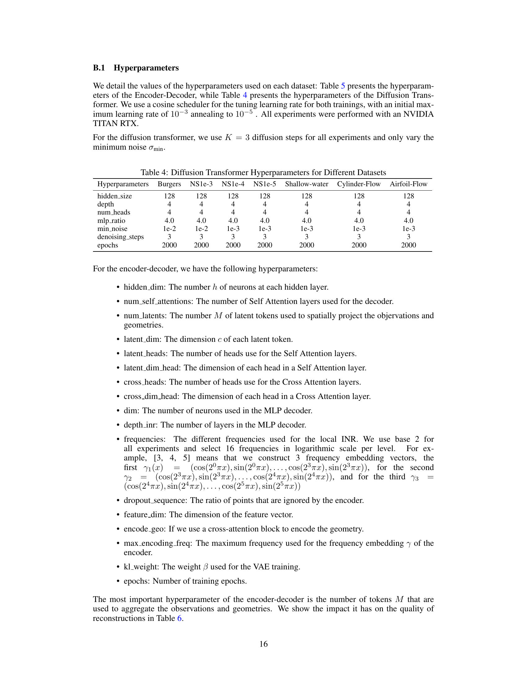
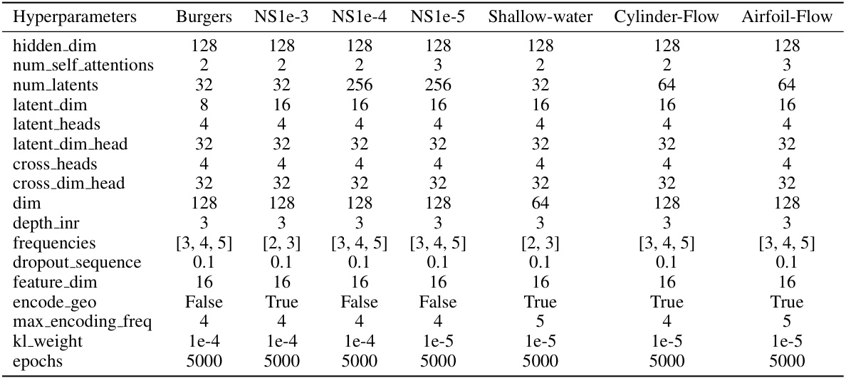
This table shows the hyperparameters used for the diffusion transformer part of the AROMA model. The hyperparameters are the same for all datasets except for the minimum noise and epochs. The table includes the hidden size, depth, number of heads, MLP ratio, minimum noise, denoising steps, and epochs.
This table compares the performance of AROMA against several baselines on three datasets: Burgers, Navier-Stokes 1e-4, and Navier-Stokes 1e-5. The performance is measured using the Relative L2 error metric, which quantifies the relative difference between the model’s predictions and the ground truth. The results demonstrate AROMA’s superior performance compared to other methods, particularly in handling turbulent phenomena.

This table presents an ablation study on the impact of varying the number of latent tokens (M) used in the model’s architecture. The results show the test reconstruction error (Relative L2 Error) for three different values of M (64, 128, and 256) on the Navier-Stokes 1 × 10⁻⁴ dataset. The data indicates an improvement in reconstruction accuracy with an increase in the number of latent tokens.

This table presents the ablation study results comparing different model variations of AROMA. The metrics used are Relative L2 errors on the test sets for Burgers, Navier-Stokes (1e-4), and Navier-Stokes (1e-5) datasets. The variations compared include AROMA with auto-encoding, AROMA without diffusion, AROMA with MLP instead of the transformer, and the full AROMA model. The results show the impact of each component on the overall performance.

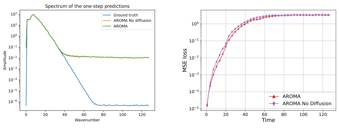
This table presents a comparison of the performance of AROMA with and without diffusion on the Kuramoto-Sivashinsky (KS) equation. The metrics used for comparison are the 1-step prediction MSE, the rollout MSE (over the entire 160 timestamps), and the duration for which the correlation between generated samples and the ground truth remains above 0.8. The results show that while the diffusion improves the rollout MSE slightly and increases the correlation duration, it does not significantly impact the overall performance on this chaotic system.
Full paper#

