TL;DR#
Conditional generation using diffusion models has emerged as a powerful technique for various applications, but existing methods suffer from limitations such as hyperparameter sensitivity and high computational costs. Many existing methods lack a unifying framework, hindering understanding and progress. This often involves issues such as being very sensitive to hyperparameters, being expensive to train, or needing access to proprietary APIs.
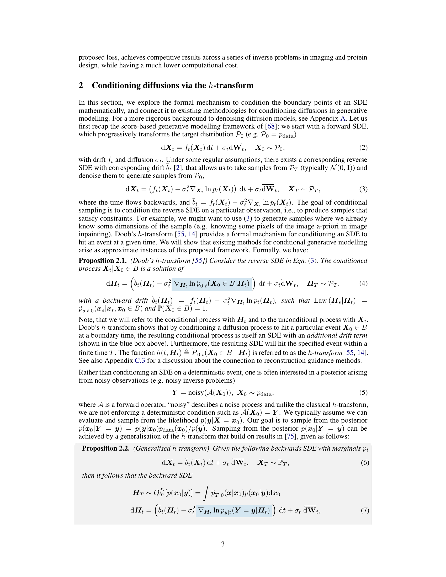
DEFT addresses these issues by using Doob’s h-transform, which provides a unified mathematical framework for conditional generation. The core contribution is a novel fine-tuning approach that learns the conditional h-transform efficiently using a small, easy-to-train network, keeping the large pre-trained model fixed. This results in substantial speed improvements and state-of-the-art performance across various benchmarks, demonstrating DEFT’s effectiveness and efficiency.
Key Takeaways#
Why does it matter?#
This paper is crucial for researchers working with diffusion models, especially those dealing with conditional generation and inverse problems. DEFT offers a significantly faster and more efficient fine-tuning method, improving upon existing approaches’ limitations in speed and hyperparameter sensitivity. This opens new avenues for applying diffusion models to various real-world tasks and inspires further research into efficient conditional generation techniques. The unified framework provided also benefits researchers in understanding and classifying different existing methods.
Visual Insights#
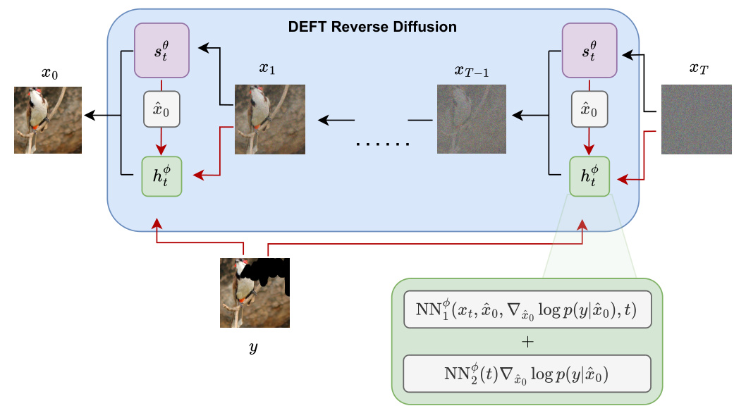
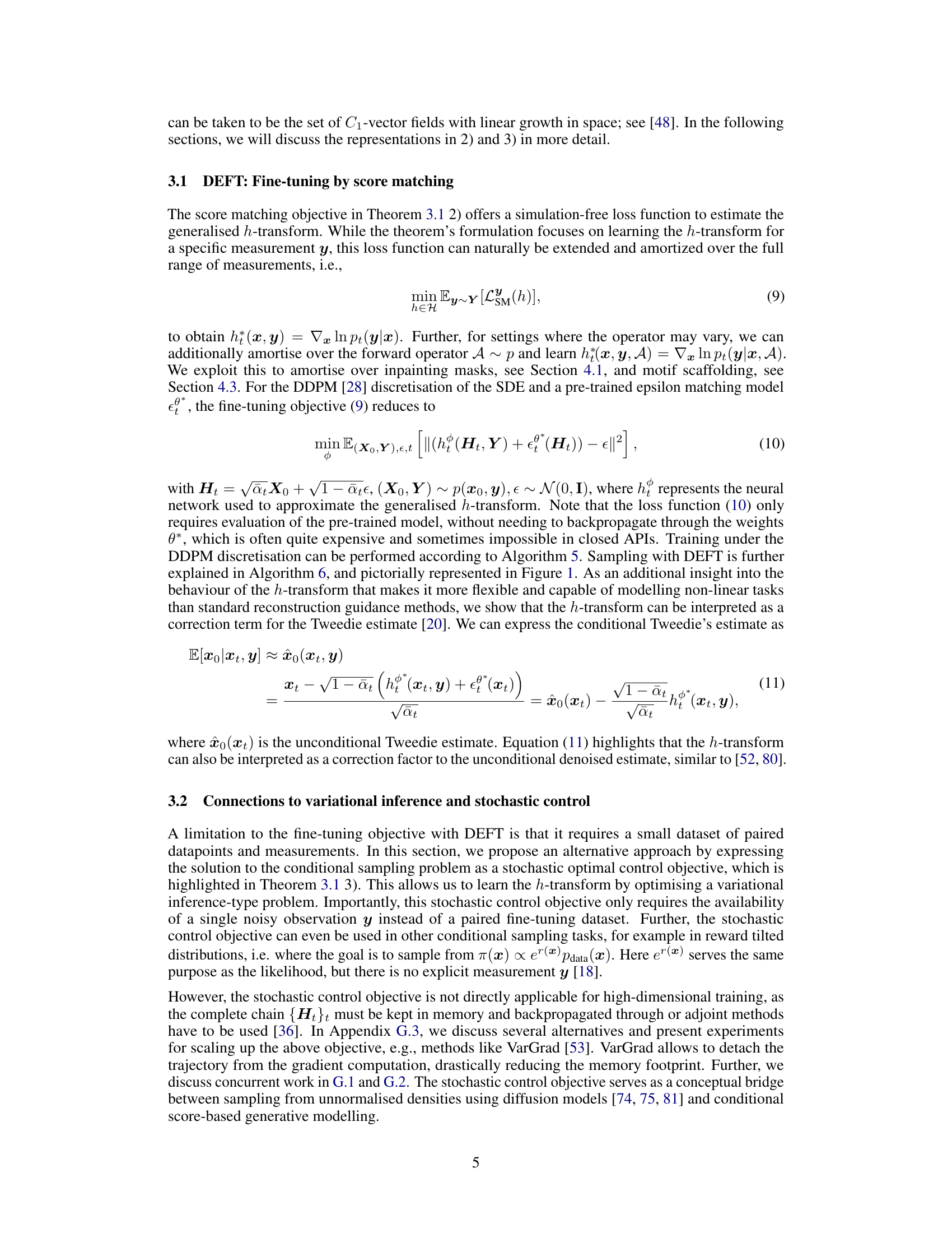
🔼 This figure illustrates the DEFT reverse diffusion process. A pre-trained unconditional diffusion model (st) and a small, fine-tuned network representing the generalized h-transform (ht) are used in each sampling step. The h-transform network incorporates a guidance term to condition the sampling process. The figure highlights the efficiency of DEFT because only the ht network needs to be trained. No backpropagation through the large pre-trained model is required during either training or sampling, leading to significant speedups.
read the caption
Figure 1: DEFT reverse diffusion setup. The pre-trained unconditional diffusion model st and the fine-tuned h-transform ht are combined at every sampling step. We propose a special network to parametrise the h-transform including the guidance term ∇ lnp(y|x̂0) as part of the architecture. Here x̂0 denotes the unconditional denoised estimate given st(xt). During training, we only need to fine-tune ht (usually 4-9% the size of st) using a small dataset of paired measurements, keeping st fixed. During sampling, we do not need to backpropagate through either model, resulting in speed-ups during evaluation.

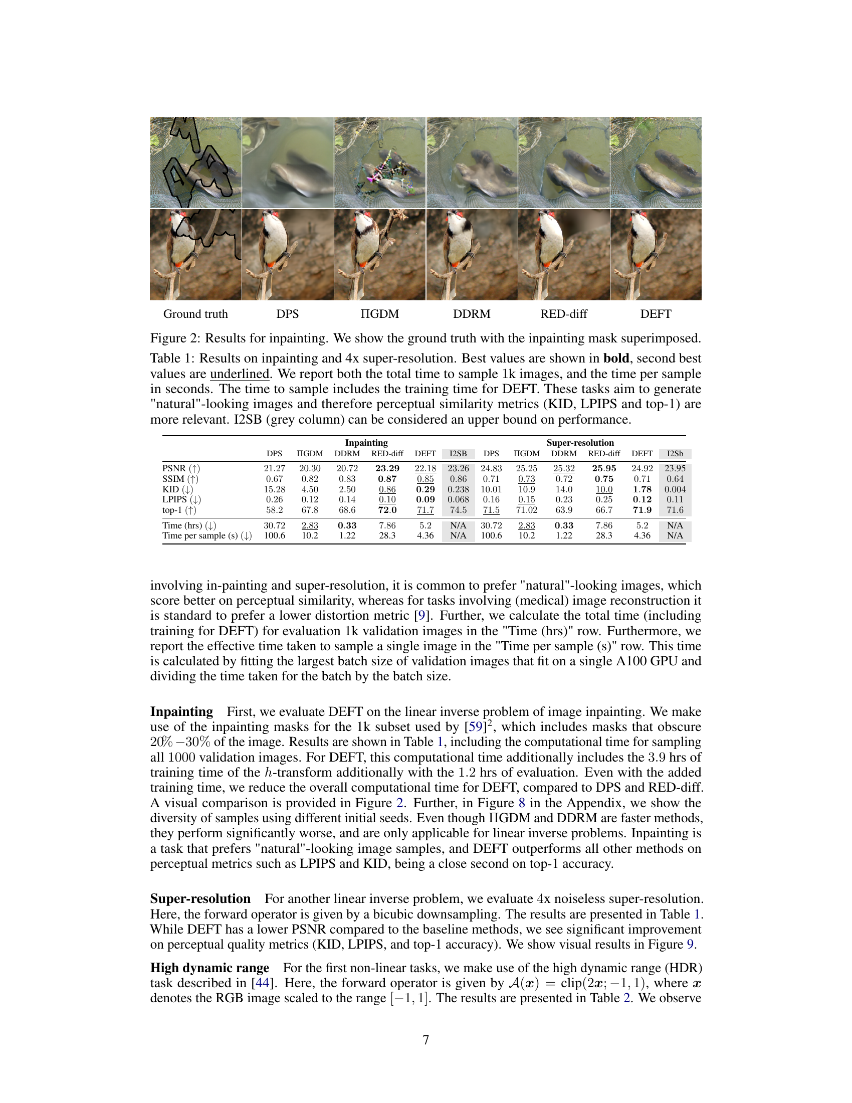
🔼 This table presents the quantitative and qualitative results of inpainting and super-resolution experiments. It compares DEFT’s performance against several baselines (DPS, IGDM, DDRM, RED-diff, and I2SB) using metrics like PSNR, SSIM, KID, LPIPS, and top-1 accuracy. Importantly, it also shows the total time and per-sample time taken for generating 1000 images, highlighting DEFT’s computational efficiency. The focus is on generating natural-looking images, making perceptual metrics more crucial than distortion metrics.
read the caption
Table 1: Results on inpainting and 4x super-resolution. Best values are shown in bold, second best values are underlined. We report both the total time to sample 1k images, and the time per sample in seconds. The time to sample includes the training time for DEFT. These tasks aim to generate \'natural\'-looking images and therefore perceptual similarity metrics (KID, LPIPS and top-1) are more relevant. I2SB (grey column) can be considered an upper bound on performance.
In-depth insights#
Doob’s h-Transform#
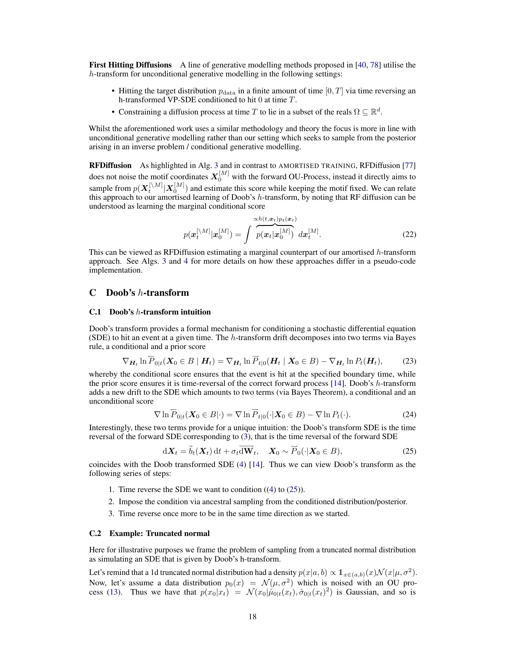
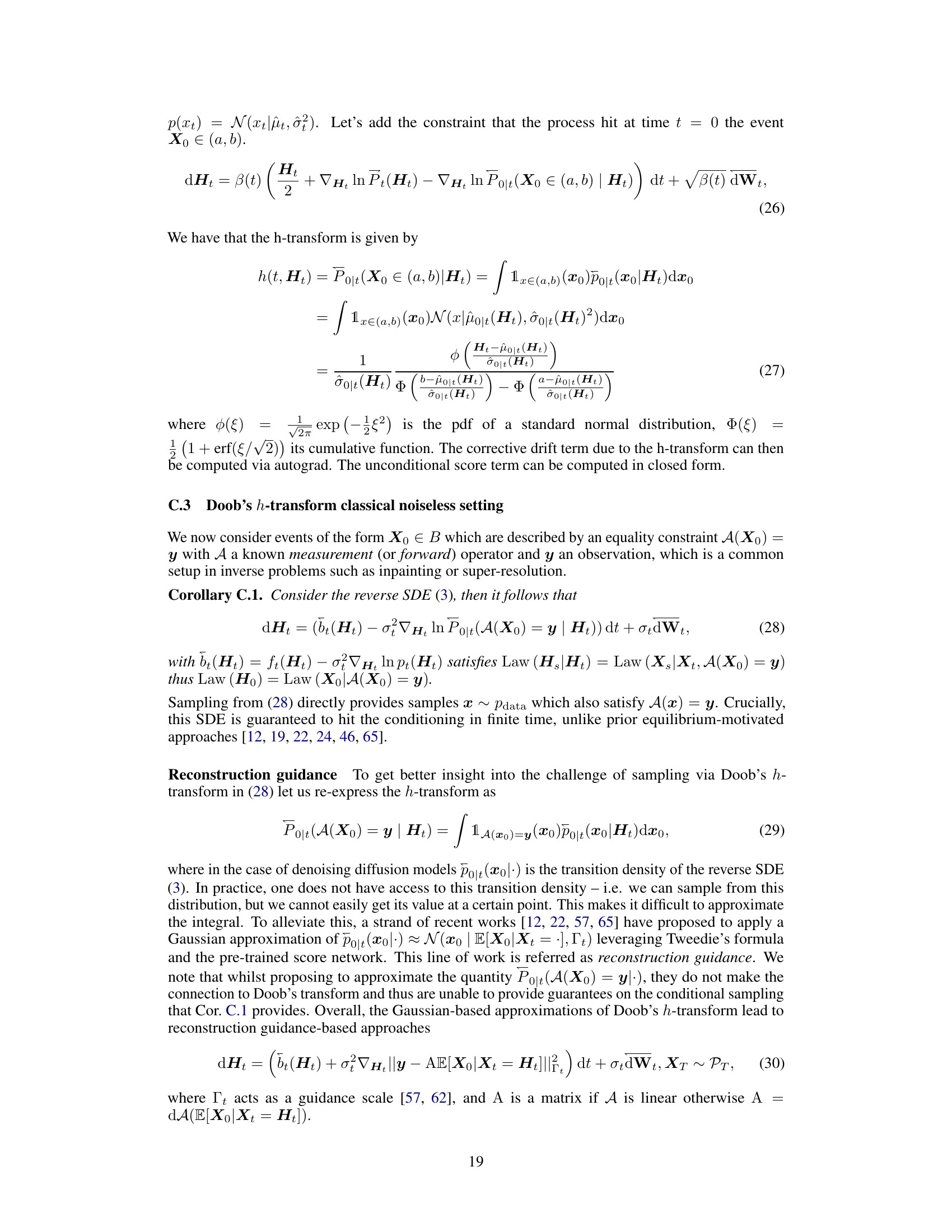
The paper leverages Doob’s h-transform, a powerful tool from stochastic calculus, to provide a unified mathematical framework for conditional sampling in diffusion models. This approach elegantly connects various existing methods, which were previously viewed as disparate, under a common umbrella. By framing conditional generation as learning a conditional h-transform, the authors introduce DEFT, a method for efficient fine-tuning. DEFT avoids the computational burden of backpropagation through large pre-trained models, thereby achieving significant speed improvements. The use of Doob’s h-transform provides theoretical guarantees about the properties of the resulting conditional process, making it a sound and principled foundation for conditional generation. Crucially, DEFT is shown to be effective across a wide range of tasks, demonstrating its versatility and applicability. The method offers a novel perspective on conditional generation and a significant improvement over existing approaches, setting a strong foundation for future research in generative modeling and inverse problems.
DEFT Fine-Tuning#
The paper introduces DEFT (Doob’s h-transform Efficient Fine-Tuning), a novel method for efficiently fine-tuning diffusion models for conditional generation. Instead of fully retraining a large model, DEFT learns a small, efficient network approximating the conditional h-transform, while keeping the pre-trained unconditional diffusion model frozen. This significantly reduces training time and computational cost. DEFT’s core strength lies in its mathematical grounding in Doob’s h-transform, unifying existing conditional generation methods under a common framework. The proposed network architecture incorporates guidance signals effectively, enabling superior performance across diverse benchmarks, including image reconstruction and protein design tasks. The approach’s simplicity and efficiency make it a powerful tool for adapting large, pre-trained models to specific conditional generation tasks while avoiding the computational burden associated with full model retraining. The results demonstrate DEFT’s superiority over existing baselines, achieving state-of-the-art performance with significant speed improvements. A key contribution is its ability to handle situations where the weights of the pre-trained model are unavailable. However, its dependence on a small fine-tuning dataset could potentially limit its generalization capabilities in certain scenarios. This limitation offers valuable directions for future exploration, including the development of more robust and sample-efficient methods.
Inverse Problem#
Inverse problems, where the goal is to infer causes from effects, are central to many scientific fields. This paper tackles inverse problems within the context of generative modeling, specifically using diffusion models. The core challenge lies in efficiently and accurately conditioning these models to reflect observed data (effects) in order to generate plausible samples of the underlying causes. Doob’s h-transform provides a powerful mathematical framework for understanding conditional generation in such settings and is used to unify existing methods. The paper addresses the limitations of prior approaches including sensitivity to hyperparameters and computational expense, proposing a novel method named DEFT (Doob’s h-transform Efficient Fine-Tuning) that leverages pre-trained unconditional models. This new approach achieves state-of-the-art results, making it a significant contribution to generative modeling of inverse problems. DEFT’s efficiency stems from fine-tuning a small network to learn the conditional transformation, thereby avoiding the need to train or backpropagate through large, pre-trained models. The resulting speed improvements and performance gains offer practical advantages across a variety of applications, demonstrating the power of this approach in solving various types of inverse problems.
Motif Scaffolding#
The research paper explores motif scaffolding within the context of protein design, leveraging the power of diffusion models. A key challenge in protein design is the creation of protein backbones that incorporate specific motifs, which are short, conserved sequences of amino acids that confer particular functions. The paper proposes a method to achieve this by conditioning a pre-trained unconditional diffusion model to generate protein sequences that incorporate a given motif. This is achieved through the use of Doob’s h-transform, a method that allows for the efficient conditioning of stochastic processes. The approach involves fine-tuning a small network to quickly learn the conditional h-transform, which enables faster training compared to existing methods. This conditional generation method is evaluated on a benchmark dataset, demonstrating competitive results and significant speedups. The results suggest that the proposed method is a promising tool for protein design and motif scaffolding, facilitating the creation of novel proteins with specific properties.
Future Work#
The paper’s lack of a dedicated ‘Future Work’ section is notable. However, considering the presented research, several promising avenues for future investigation emerge. Extending DEFT to more complex and higher-dimensional inverse problems beyond image reconstruction and protein design is crucial. Exploring its applicability to other modalities like medical imaging or other scientific domains would significantly broaden its impact. Furthermore, investigating the effectiveness of DEFT with various model architectures and loss functions would help refine the algorithm’s performance and applicability. Given that DEFT prioritizes efficiency, exploring efficient training strategies, such as transfer learning from similar domains or leveraging self-supervised learning techniques, may be beneficial. Additionally, a more thorough investigation into the theoretical properties of the generalised h-transform, including its limitations and generalizability, would provide deeper understanding and further guide algorithm development. Finally, a comprehensive comparison of DEFT’s performance against a wider range of state-of-the-art conditional generation methods is necessary to establish its broader standing within the field.
More visual insights#
More on figures

🔼 This figure shows the results of an inpainting task, comparing different methods (DPS, IGDM, DDRM, RED-diff, and DEFT) against the ground truth. The images demonstrate the effectiveness of each method at filling in missing parts of an image based on the provided context. The superimposed inpainting mask highlights the regions that were missing in the original images.
read the caption
Figure 2: Results for inpainting. We show the ground truth with the inpainting mask superimposed.
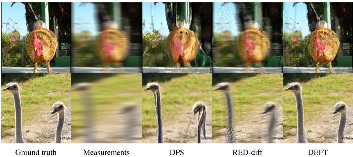
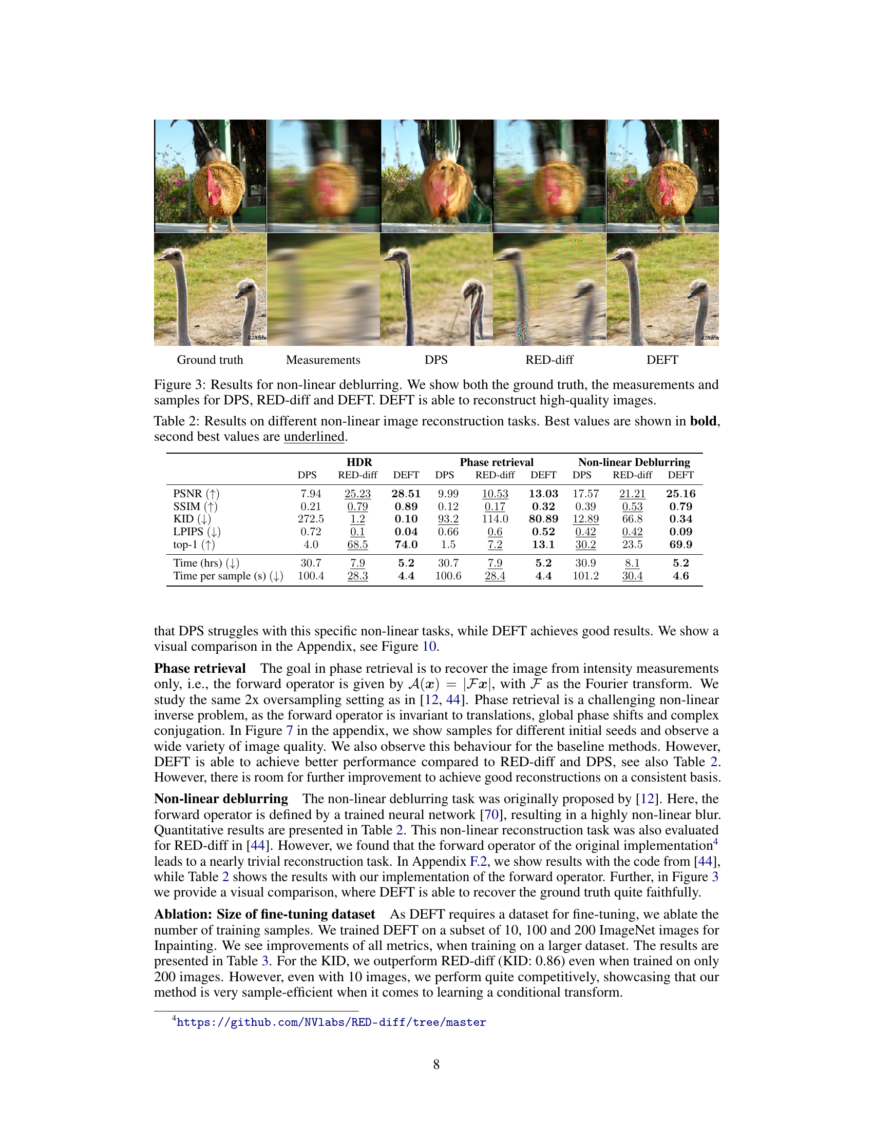
🔼 This figure shows a comparison of the results of different methods on a non-linear deblurring task. The top row displays a chicken image: the ground truth, the blurry measurements, and the reconstructed images from DPS, RED-diff, and DEFT. The bottom row shows the same comparison but with an ostrich image. The figure visually demonstrates that DEFT produces higher quality reconstructed images compared to the other methods.
read the caption
Figure 3: Results for non-linear deblurring. We show both the ground truth, the measurements and samples for DPS, RED-diff and DEFT. DEFT is able to reconstruct high-quality images.

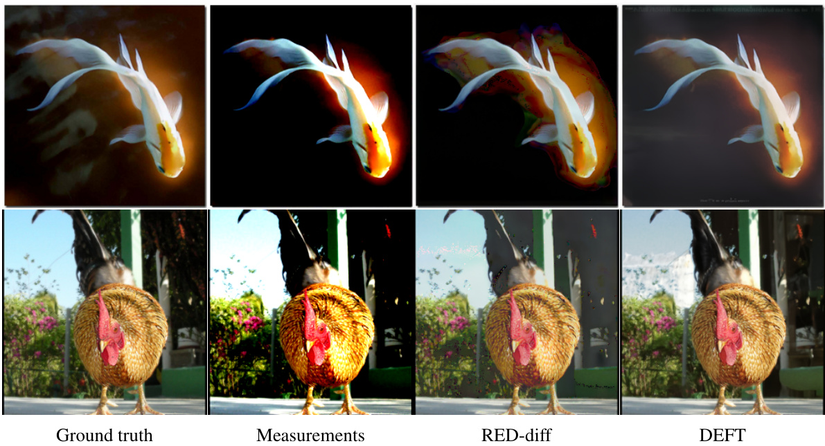
🔼 This figure shows the ground truth and the reconstructions generated by DPS, RED-diff, and DEFT for computed tomography on the LoDoPab-CT dataset. It visually demonstrates the performance of each method in reconstructing the image from noisy measurements. DEFT shows superior performance compared to other methods.
read the caption
Figure 4: Reconstructions for computed tomography on LoDoPab-CT

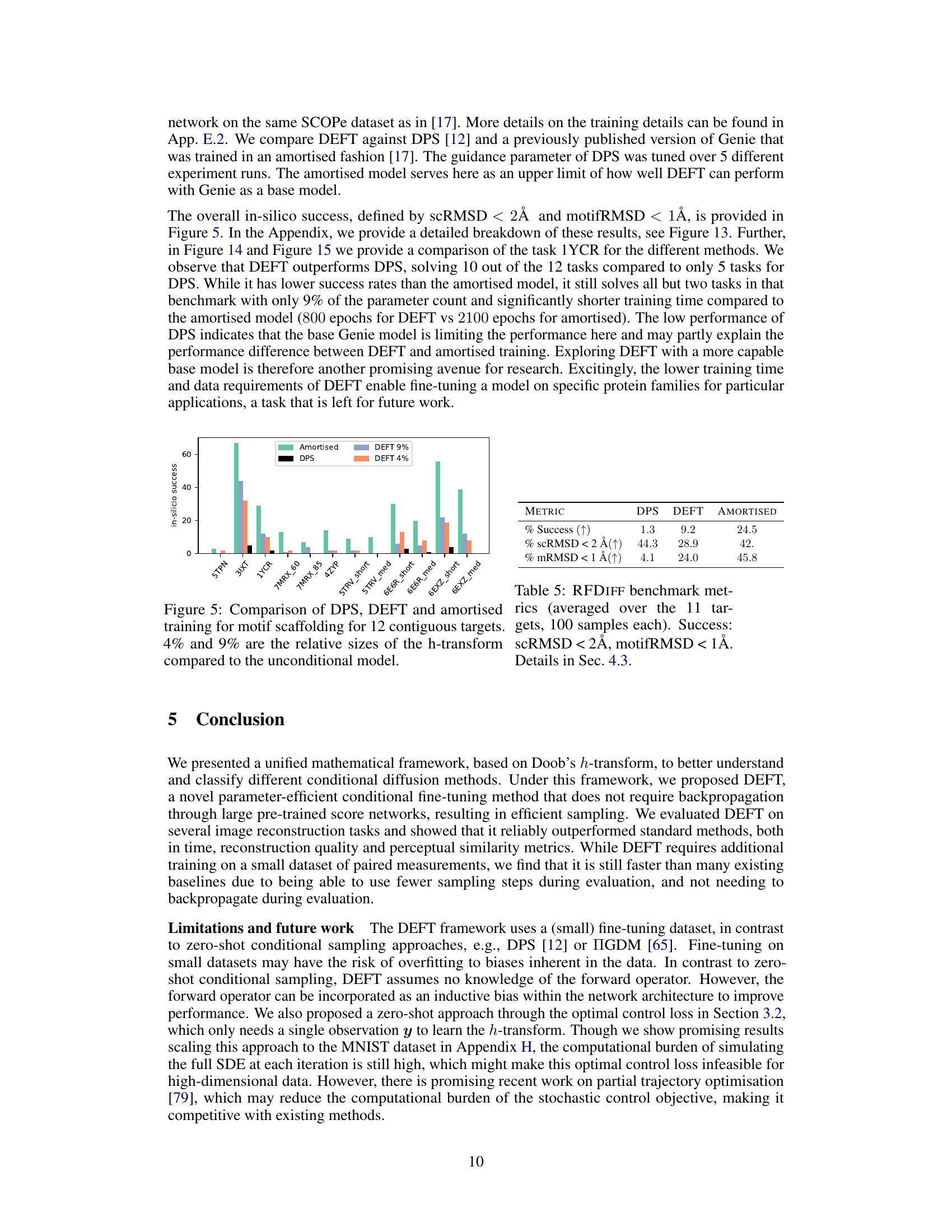
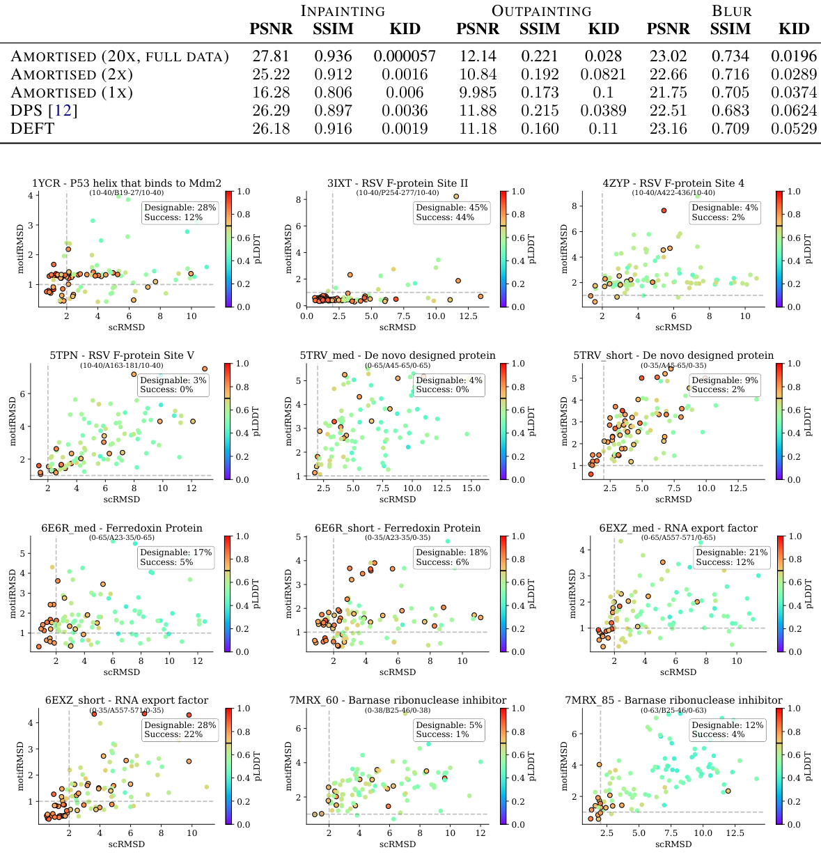
🔼 This figure shows a bar chart comparing the in-silico success rates of three different methods for motif scaffolding: DPS, DEFT with a small network (4% of the size of the unconditional model), and DEFT with a larger network (9% of the size of the unconditional model). The x-axis represents the 12 different contiguous target protein motifs tested, and the y-axis shows the percentage of successful motif scaffolds generated by each method. The figure highlights that DEFT, even with a small network, significantly outperforms DPS. The amortised method achieves higher success rates overall but requires more parameters and training.
read the caption
Figure 5: Comparison of DPS, DEFT and amortised training for motif scaffolding for 12 contiguous targets. 4% and 9% are the relative sizes of the h-transform compared to the unconditional model.

🔼 This figure illustrates the DEFT reverse diffusion process. A pre-trained unconditional diffusion model and a small, fine-tuned network (the h-transform) are combined at each step of the sampling process. The h-transform network is trained using a small dataset to learn a conditional transformation while leaving the main model unchanged. This setup allows for fast conditional generation without backpropagation through the main model, leading to speed improvements.
read the caption
Figure 1: DEFT reverse diffusion setup. The pre-trained unconditional diffusion model st and the fine-tuned h-transform hi are combined at every sampling step. We propose a special network to parametrise the h-transform including the guidance term ∇ lnp(y|20) as part of the architecture. Here 20 denotes the unconditional denoised estimate given sf(xt). During training, we only need to fine-tune hi (usually 4-9% the size of st) using a small dataset of paired measurements, keeping so fixed. During sampling, we do not need to backpropagate through either model, resulting in speed-ups during evaluation.

🔼 This figure illustrates the architecture of the DEFT reverse diffusion process. The pre-trained unconditional diffusion model and a smaller, fine-tuned h-transform network are combined at each step of the sampling process. The h-transform network, parameterized to include a guidance term, is significantly smaller than the unconditional model (4-9%). Crucially, the figure highlights that training only requires fine-tuning the h-transform, leaving the larger pre-trained model unchanged, and during sampling, backpropagation through either model is unnecessary, leading to faster inference.
read the caption
Figure 1: DEFT reverse diffusion setup. The pre-trained unconditional diffusion model st and the fine-tuned h-transform his are combined at every sampling step. We propose a special network to parametrise the h-transform including the guidance term ∇ lnp(y|20) as part of the architecture. Here 20 denotes the unconditional denoised estimate given sf(xt). During training, we only need to fine-tune hi (usually 4-9% the size of st) using a small dataset of paired measurements, keeping so fixed. During sampling, we do not need to backpropagate through either model, resulting in speed-ups during evaluation.

🔼 This figure displays the results of an inpainting task using different methods including DEFT. The ground truth image is shown alongside the results obtained by DPS, IGDM, DDRM, RED-diff, and DEFT. Each image shows the result of inpainting where part of the image is missing or obscured by a mask. The comparison allows a visual assessment of the effectiveness of each method in restoring the missing portions of the image while maintaining image quality.
read the caption
Figure 2: Results for inpainting. We show the ground truth with the inpainting mask superimposed.

🔼 This figure shows the results of an inpainting task, where a portion of an image is missing. The ground truth image is shown alongside the results from different methods (DPS, IGDM, DDRM, RED-diff, and DEFT). The superimposed mask highlights the area that was originally missing and needed to be inpainted by the different algorithms.
read the caption
Figure 2: Results for inpainting. We show the ground truth with the inpainting mask superimposed.

🔼 This figure shows the results of an inpainting experiment. The top row shows the results for one image and the bottom row shows the results for another image. Each row displays the ground truth image (leftmost), followed by the results generated using DPS, IGDM, DDRM, RED-diff, and DEFT methods. The inpainting masks used are superimposed on the ground truth images, showing the regions where the model was tasked with filling in missing image information. The images demonstrate the different methods’ abilities to reconstruct natural-looking details within the masked regions.
read the caption
Figure 2: Results for inpainting. We show the ground truth with the inpainting mask superimposed.
🔼 This figure shows the results of an inpainting task. The top row displays the ground truth images, with the inpainting masks superimposed to show the regions that were missing. The bottom four rows depict the inpainting results generated by four different methods: DPS, IGDM, DDRM, RED-diff, and DEFT. Each column represents a different image and provides a visual comparison of the performance of the different methods in reconstructing the missing parts of the image. The figure demonstrates DEFT’s ability to produce high-quality inpainting results that are visually similar to the ground truth.
read the caption
Figure 2: Results for inpainting. We show the ground truth with the inpainting mask superimposed.
🔼 This figure illustrates the architecture of DEFT (Doob’s h-transform Efficient Fine-Tuning), a method for conditional generation using diffusion models. A pre-trained unconditional diffusion model is combined with a smaller, fine-tuned network (h-transform) to generate conditional samples. The h-transform network incorporates guidance information to direct the sampling process towards the desired condition. The figure highlights that during training, only the h-transform is updated, leaving the larger unconditional model unchanged, leading to faster training times. Similarly, during sampling, backpropagation is only needed for the smaller network, resulting in faster sampling.
read the caption
Figure 1: DEFT reverse diffusion setup. The pre-trained unconditional diffusion model s and the fine-tuned h-transform h are combined at every sampling step. We propose a special network to parametrise the h-transform including the guidance term ∇ lnp(y|z0) as part of the architecture. Here z0 denotes the unconditional denoised estimate given sf(xt). During training, we only need to fine-tune h (usually 4-9% the size of s) using a small dataset of paired measurements, keeping s fixed. During sampling, we do not need to backpropagate through either model, resulting in speed-ups during evaluation.

🔼 This figure illustrates the architecture of DEFT, a method for efficient fine-tuning of diffusion models. It shows how a pre-trained unconditional diffusion model is combined with a small, fine-tuned network (the h-transform) at each step of the reverse diffusion process. The h-transform is trained on a small dataset of paired measurements, and its inclusion allows for faster sampling and improved conditional generation without requiring backpropagation through the larger model.
read the caption
Figure 1: DEFT reverse diffusion setup. The pre-trained unconditional diffusion model st and the fine-tuned h-transform his are combined at every sampling step. We propose a special network to parametrise the h-transform including the guidance term ∇ lnp(y|20) as part of the architecture. Here 20 denotes the unconditional denoised estimate given sf(xt). During training, we only need to fine-tune hi (usually 4-9% the size of st) using a small dataset of paired measurements, keeping so fixed. During sampling, we do not need to backpropagate through either model, resulting in speed-ups during evaluation.
🔼 This figure illustrates the architecture of the DEFT reverse diffusion process. It shows how a pre-trained unconditional diffusion model and a small fine-tuned network are combined to perform conditional generation. The figure highlights the key components of the process, including the h-transform, the guidance term, and the training and sampling steps. It also emphasizes the efficiency of DEFT by showing that only a small network needs to be fine-tuned, while keeping the larger unconditional network fixed. This results in significant speedups during evaluation.
read the caption
Figure 1: DEFT reverse diffusion setup. The pre-trained unconditional diffusion model st and the fine-tuned h-transform hi are combined at every sampling step. We propose a special network to parametrise the h-transform including the guidance term ∇ lnp(y|20) as part of the architecture. Here 20 denotes the unconditional denoised estimate given sf(xt). During training, we only need to fine-tune hi (usually 4-9% the size of st) using a small dataset of paired measurements, keeping st fixed. During sampling, we do not need to backpropagate through either model, resulting in speed-ups during evaluation.

🔼 This figure illustrates the DEFT reverse diffusion process. It shows how a pre-trained unconditional diffusion model is combined with a small, fine-tuned network (the h-transform) at each step of the sampling process. The h-transform network incorporates the guidance term (∇ lnp(y|20)) to condition the generation. The diagram highlights that only the h-transform requires training, using a small dataset. Importantly, during sampling, backpropagation isn’t needed through either network, enabling faster inference.
read the caption
Figure 1: DEFT reverse diffusion setup. The pre-trained unconditional diffusion model st and the fine-tuned h-transform his are combined at every sampling step. We propose a special network to parametrise the h-transform including the guidance term ∇ lnp(y|20) as part of the architecture. Here 20 denotes the unconditional denoised estimate given sf(xt). During training, we only need to fine-tune hi (usually 4-9% the size of st) using a small dataset of paired measurements, keeping so fixed. During sampling, we do not need to backpropagate through either model, resulting in speed-ups during evaluation.

🔼 This figure illustrates the reverse diffusion process used in the DEFT model. The process combines a pre-trained unconditional diffusion model (st) with a fine-tuned, smaller h-transform network (hi) at each step. The h-transform network is designed to efficiently learn the conditional distribution, using the gradient of the log-likelihood (∇ lnp(y|20)) as part of its architecture. The figure highlights that only hi needs to be trained, with st remaining unchanged, resulting in faster training and sampling speeds due to avoiding backpropagation through the large st model during inference.
read the caption
Figure 1: DEFT reverse diffusion setup. The pre-trained unconditional diffusion model st and the fine-tuned h-transform hi are combined at every sampling step. We propose a special network to parametrise the h-transform including the guidance term ∇ lnp(y|20) as part of the architecture. Here 20 denotes the unconditional denoised estimate given sf(xt). During training, we only need to fine-tune hi (usually 4-9% the size of st) using a small dataset of paired measurements, keeping so fixed. During sampling, we do not need to backpropagate through either model, resulting in speed-ups during evaluation.
More on tables

🔼 This table presents the quantitative results for three non-linear image reconstruction tasks: High Dynamic Range (HDR) imaging, phase retrieval, and non-linear deblurring. For each task, it compares the performance of three methods: DPS, RED-diff, and DEFT. The metrics used are PSNR, SSIM, KID, LPIPS, and top-1 accuracy, along with the total training time and time per sample. The best and second-best results for each metric are highlighted in bold and underlined, respectively, for easy comparison across the methods.
read the caption
Table 2: Results on different non-linear image reconstruction tasks. Best values are shown in bold, second best values are underlined.
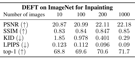
🔼 This table shows the performance of DEFT on ImageNet inpainting task with different sizes of the fine-tuning dataset. The metrics used are PSNR, SSIM, KID, LPIPS, and top-1 accuracy. The results demonstrate that DEFT achieves competitive results even with small training datasets, indicating its sample efficiency.
read the caption
Table 3: Varying the size of the fine-tuning dataset for DEFT for Inpainting on ImageNet.

🔼 This table presents the quantitative results of computed tomography image reconstruction experiments on two datasets, AAPM and LoDoPab-CT. The results are shown for three methods: DEFT, DPS, and RED-diff. The metrics include PSNR (Peak Signal-to-Noise Ratio), SSIM (Structural Similarity Index), and the time taken to generate a single image. DEFT uses 100 DDIM (Denoising Diffusion Implicit Models) sampling steps, while the other two methods use 1000 steps. Best results are bolded, and second-best results are underlined. The table highlights the superior performance and efficiency of the proposed DEFT method.
read the caption
Table 4: Results for CT on AAPM and LODOPAB-CT and sampling time per image on a single GeForce RTX 3090. Best values are shown in bold, second best values are underlined. For DEFT we use 100 DDIM steps, while RED-diff and DPS use 1000 time steps.
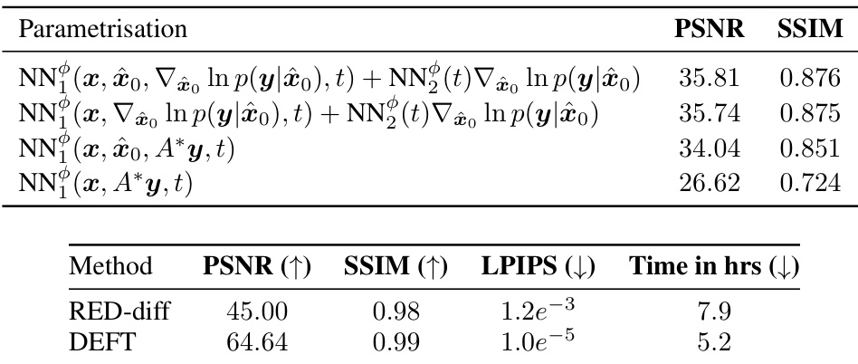
🔼 This table presents quantitative results for image inpainting and 4x super-resolution tasks. It compares DEFT’s performance against several other methods (DPS, IGDM, DDRM, RED-diff, and I2SB). Metrics include PSNR, SSIM, KID, LPIPS, and top-1 accuracy, reflecting both objective image quality and perceptual similarity. The table also shows the total time and time per sample required for generating 1,000 images. I2SB, trained on the full ImageNet dataset, serves as a performance upper bound.
read the caption
Table 1: Results on inpainting and 4x super-resolution. Best values are shown in bold, second best values are underlined. We report both the total time to sample 1k images, and the time per sample in seconds. The time to sample includes the training time for DEFT. These tasks aim to generate \'natural\'-looking images and therefore perceptual similarity metrics (KID, LPIPS and top-1) are more relevant. I2SB (grey column) can be considered an upper bound on performance.
Full paper#


