↗ OpenReview ↗ NeurIPS Homepage ↗ Chat
TL;DR#
Many anomaly detection methods struggle with incomplete datasets, which are extremely common in real-world applications. Simply imputing missing values before detection often introduces bias, leading to inaccurate results. This is particularly problematic in unsupervised learning scenarios where you only have normal data for training. The method of filling missing values with mean or median, followed by the application of existing anomaly detection methods, was shown to be ineffective.
To solve this, the researchers developed ImAD, a new method that tackles data imputation and anomaly detection simultaneously. ImAD creates “pseudo-abnormal” samples to correct for biases in imputation models trained on only normal data. The method is shown to be effective with both theoretical guarantees and experimental results that consistently outperformed other state-of-the-art methods across different datasets, demonstrating improved accuracy and reduced bias in anomaly detection with incomplete data.
Key Takeaways#
Why does it matter?#
This paper is crucial because it directly addresses the prevalent issue of missing data in anomaly detection, a common challenge across many scientific and engineering domains. The proposed ImAD method offers a significant advancement by integrating data imputation and anomaly detection into a unified framework, improving accuracy and mitigating biases inherent in previous two-stage approaches. This opens avenues for more reliable anomaly detection in various applications dealing with incomplete data, which is highly relevant to current research trends.
Visual Insights#
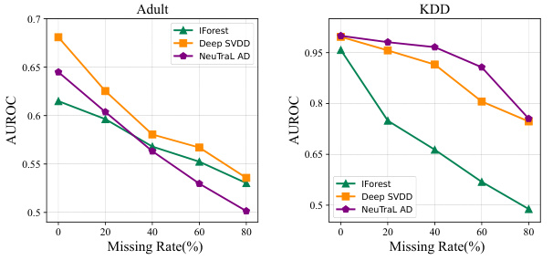
This figure shows the Area Under the Receiver Operating Characteristic (AUROC) curves for four different anomaly detection methods (IForest, Deep SVDD, NeuTraL AD) on two datasets (Adult and KDD). The x-axis represents the missing data rate (percentage), and the y-axis represents the AUROC score. The lines show how the accuracy of each method decreases as the amount of missing data increases. This illustrates the challenge of applying standard anomaly detection techniques to datasets with missing values.

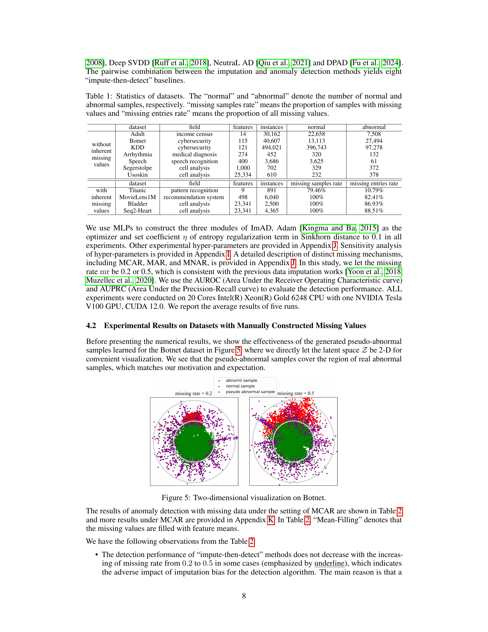
This table presents the characteristics of eleven datasets used in the experiments. Each dataset’s field, number of features, total number of instances, the number of normal instances, and the number of abnormal instances are listed. For datasets with inherent missing values, the missing sample rate (percentage of samples with missing values) and missing entry rate (percentage of all entries that are missing) are provided. The datasets are categorized into those without inherent missing values and those with inherent missing values.
In-depth insights#
Imputation Bias#
Imputation bias, in the context of anomaly detection, specifically refers to the distortion introduced when imputation methods, trained solely on normal data, are applied to incomplete anomaly instances. This leads to imputed values that skew towards normality, obscuring the anomalous characteristics that would otherwise be readily detectable. The core problem lies in the inability of models trained on normal data to correctly extrapolate the characteristics of anomalous, incomplete data, resulting in inaccurate imputation. This creates a significant challenge because anomaly detection methods rely on the accuracy of these imputed values. Consequently, methods that directly incorporate imputation and anomaly detection into a unified optimization framework are likely to mitigate this bias by allowing both processes to influence each other during learning, resulting in more accurate detection of anomalies despite missing values.
ImAD Framework#
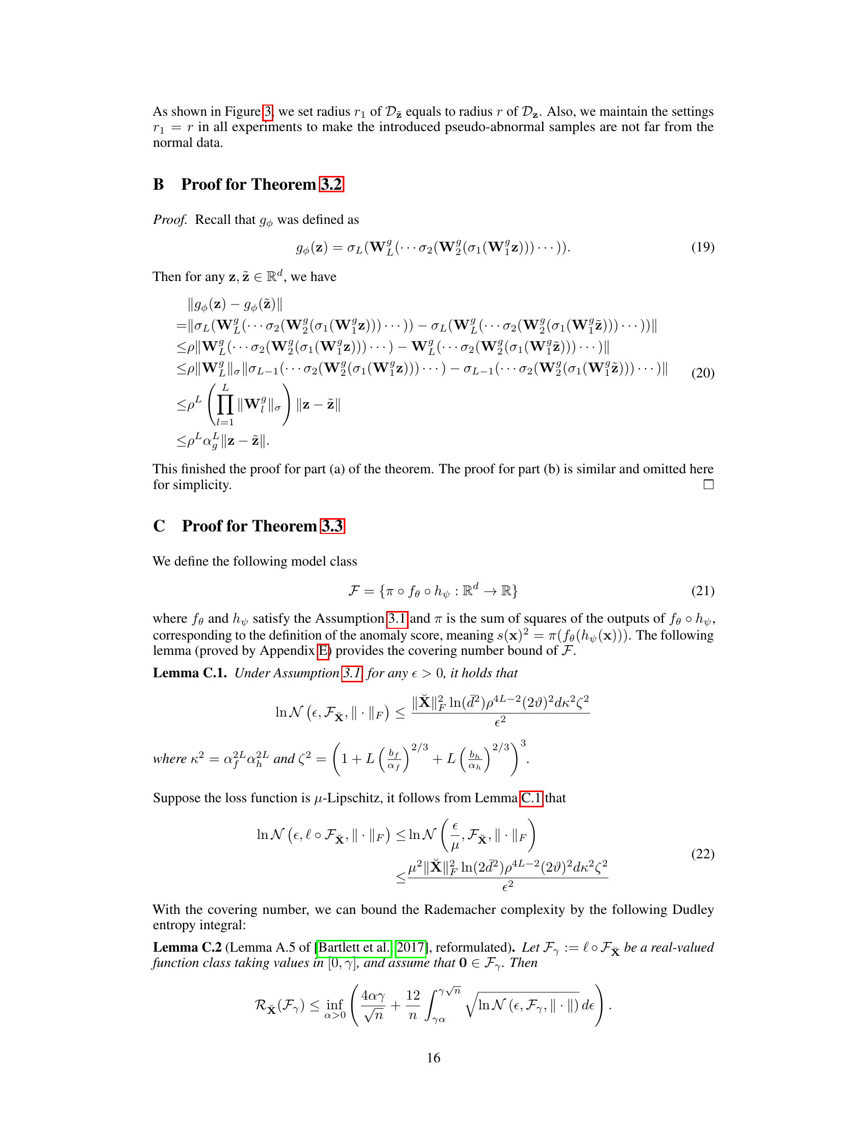
The ImAD framework, designed for unsupervised anomaly detection with missing values, integrates data imputation and anomaly detection. Its key innovation is the generation of pseudo-abnormal samples to mitigate imputation bias. This is achieved by training an imputation model I, a projector P mapping data to a latent space, and a reconstructor R mapping the latent space back to the original data space. The model learns to generate pseudo-abnormal samples in the latent space and then uses the imputation model to fill in any missing data in both the normal and pseudo-abnormal samples. By training the model on both types of data, the framework addresses the limitation of imputation models trained only on normal data, thereby improving the robustness and accuracy of anomaly detection in datasets with incomplete entries. The framework’s end-to-end nature ensures optimal coordination between the imputation and detection processes, addressing the shortcomings of the traditional two-stage “impute-then-detect” approach. Theoretical guarantees are provided to support its effectiveness.
Theoretical Guarantees#
A theoretical guarantee section in a research paper on anomaly detection with missing values would ideally provide a rigorous mathematical justification for the algorithm’s effectiveness. This would likely involve proving bounds on the probability of correct anomaly detection, perhaps under specific assumptions about the data distribution and the missing data mechanism. Key aspects to look for would include: statements on the algorithm’s consistency (does it converge to the true solution as the amount of data grows?), its generalization ability (how well does it perform on unseen data?), and the impact of the missing data on its performance. Proof techniques might include concentration inequalities, covering numbers, or other tools from statistical learning theory. The strength of the guarantees would depend heavily on the stringency of the assumptions made; weaker assumptions would lead to more general but potentially looser bounds, while stronger assumptions could enable tighter bounds but limit the scope of applicability. A well-written section would clearly state all assumptions and discuss their implications for the practical use of the algorithm. Importantly, it should highlight the difference between theoretical guarantees and empirical results, emphasizing the importance of experimental validation.
Missing Data Types#
The concept of “Missing Data Types” is crucial in data analysis and machine learning, especially concerning the reliability and validity of results. There are several categories to consider including Missing Completely at Random (MCAR) where the probability of missingness is unrelated to any observed or unobserved data. Missing at Random (MAR) is a more nuanced scenario; the probability of missingness depends on other observed data, but not the missing values themselves. Missing Not at Random (MNAR) represents the most challenging situation where the probability of missingness is directly related to the values that are missing, potentially introducing significant bias. Handling missing data requires careful consideration of its type. Inappropriate handling, such as simple imputation with means or medians without considering the missing data mechanism, can significantly affect the accuracy and robustness of model training and downstream analyses. Therefore, selecting appropriate imputation techniques or modeling approaches that explicitly address the specific missing data type is essential for trustworthy and accurate results. Advanced imputation methods such as multiple imputation and generative models are often employed to mitigate the impact of MNAR data. Rigorous evaluation of imputation techniques is necessary to determine which approach is best suited for specific datasets and analyses.
Future Directions#
Future research could explore extending the proposed ImAD framework to handle various data modalities beyond tabular data, such as images and time series. Addressing the inherent challenges posed by different data structures and missing data mechanisms within these modalities would be crucial. Furthermore, investigating the theoretical properties of ImAD under more relaxed assumptions, potentially proving its effectiveness with weaker conditions, is important. Developing more efficient and scalable versions of ImAD, perhaps through architectural modifications or algorithmic optimizations, would be highly beneficial for real-world applications involving large datasets. Finally, thorough empirical evaluations on diverse, real-world datasets with varied missing data patterns are needed to validate the generalizability and robustness of the method. The impact of different imputation techniques and anomaly detection algorithms on ImAD’s performance should also be investigated.
More visual insights#
More on figures

This figure shows the recall rate degradation of different anomaly detection methods when using the naive imputation strategy (mean or median imputation) and state-of-the-art imputation methods (MissForest and GAIN) on two real-world datasets (Adult and KDD). The results demonstrate that the naive strategy significantly reduces the recall rate as the missing data rate increases, while even the advanced imputation methods still suffer from imputation bias, leading to lower recall rates on the abnormal data. The key observation is the negative effect of imputation bias in unsupervised anomaly detection when the training data consist solely of normal samples. The impute-then-detect methods yield lower recall rates compared to using complete data, highlighting the challenge posed by imputation bias in anomaly detection tasks.

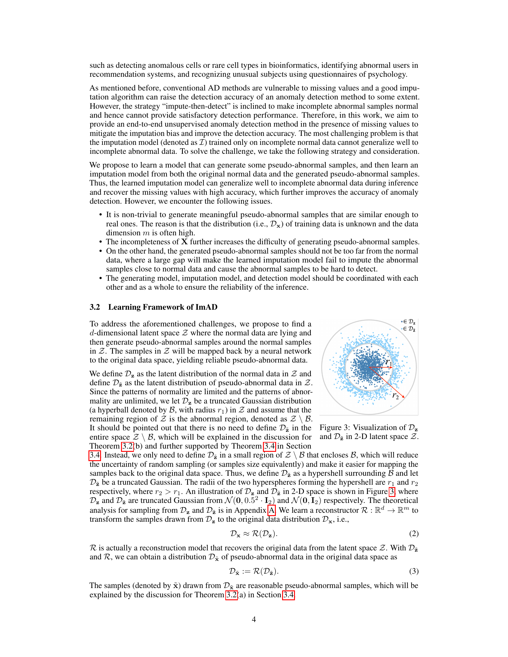
This figure visualizes the latent distributions Dz and Dž in a two-dimensional latent space Z. Dz represents the latent distribution of normal data, shown as a cluster of dark blue points concentrated near the origin. Dž represents the latent distribution of pseudo-abnormal samples, which are generated by the ImAD model to mitigate imputation bias. These are shown as lighter blue points forming a ring around Dz. The figure illustrates how ImAD generates pseudo-abnormal samples in the latent space, ensuring that they are distinct from normal data while remaining relatively close to enhance the model’s ability to distinguish between normal and abnormal samples.
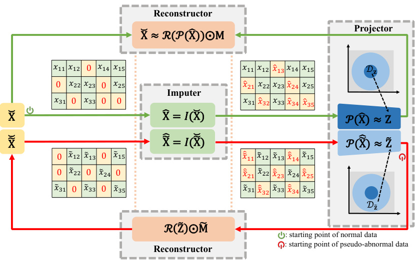
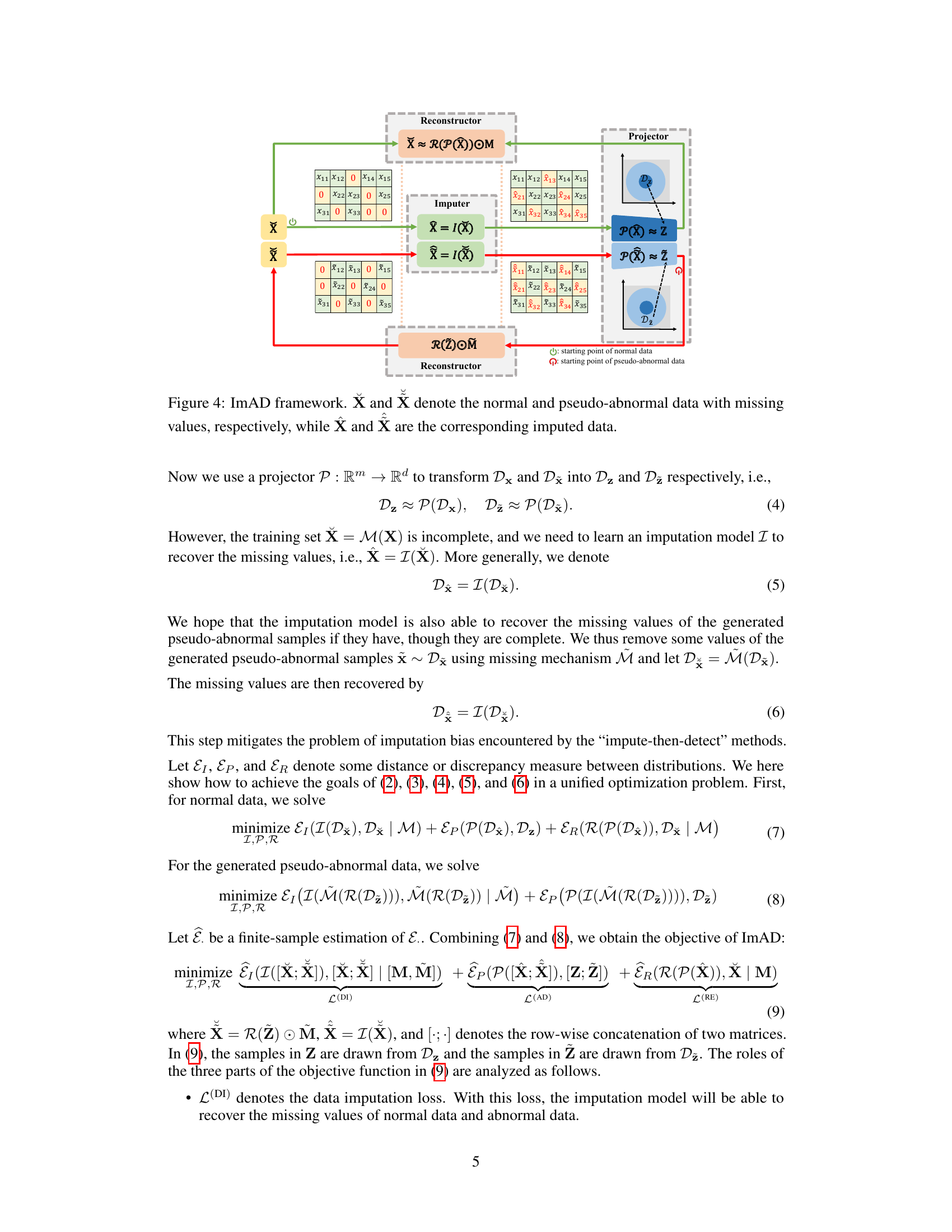
This figure illustrates the ImAD framework, showing how normal and pseudo-abnormal data with missing values are processed. The normal data (X) and pseudo-abnormal data (X) are first imputed using an imputer (I) to fill in missing values, resulting in imputed data (X) and (X). These imputed datasets are then projected into a lower-dimensional latent space (Z) using a projector (P). The pseudo-abnormal data is generated based on the latent representations of normal data. Finally, a reconstructor (R) maps the latent space representations back to the original data space to create pseudo-abnormal samples, which are then combined with the original normal samples for anomaly detection.
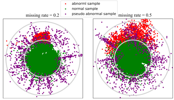
This figure visualizes the effectiveness of the generated pseudo-abnormal samples learned by the ImAD model for the Botnet dataset. The 2D latent space is shown with three types of samples: real normal samples (green), real abnormal samples (red), and the generated pseudo-abnormal samples (purple). The visualization shows that the pseudo-abnormal samples effectively cover the region of real abnormal samples, which supports the ImAD’s mechanism in mitigating imputation bias by filling in missing values for abnormal samples.
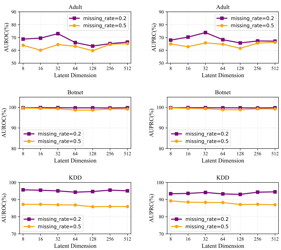
The figure visualizes the performance of anomaly detection on three datasets (Adult, Botnet, KDD) across various latent dimensions. Separate plots display AUROC and AUPRC for each dataset, at two different missing rates (0.2 and 0.5). The x-axis represents the latent dimension, while the y-axis shows the AUROC and AUPRC values, respectively. This allows for a comparison of model performance in different latent spaces and under different data completeness conditions.

This figure visualizes the results of anomaly detection on the Botnet dataset in a 2D latent space. It shows the distribution of normal samples, abnormal samples, and pseudo-abnormal samples generated by the ImAD model. The pseudo-abnormal samples effectively cover the region of real abnormal samples, which demonstrates the model’s ability to generate realistic pseudo-abnormal data for mitigating imputation bias and improving the accuracy of anomaly detection.
This figure visualizes the latent space Z (reduced to 2D for visualization) of the Botnet dataset. It shows the distribution of normal samples (blue), abnormal samples (red), and pseudo-abnormal samples generated by ImAD (green) for missing rates of 0.2 and 0.5. The visualization demonstrates that the pseudo-abnormal samples effectively cover the region occupied by the real abnormal samples, indicating the method’s ability to generate meaningful pseudo-abnormal data that helps mitigate imputation bias.

This figure visualizes the performance of the ImAD model on three datasets (Adult, Botnet, and KDD) across various latent dimensions. It shows how the AUROC and AUPRC metrics change as the dimensionality of the latent space used in the ImAD model varies. This helps demonstrate the model’s robustness and sensitivity to changes in the latent space’s dimensionality and its implications for the accuracy of anomaly detection.

The figure shows the performance of AUROC and AUPRC on three datasets (Adult, Botnet, and KDD) with different latent dimensions (d). The x-axis represents the latent dimension, while the y-axis represents the AUROC and AUPRC values. Separate lines are shown for the different missing rates (0.2 and 0.5). The figure illustrates how the choice of latent dimension impacts the performance of the anomaly detection model in the presence of missing data.
More on tables
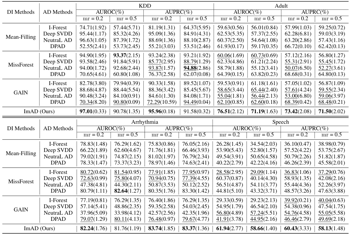
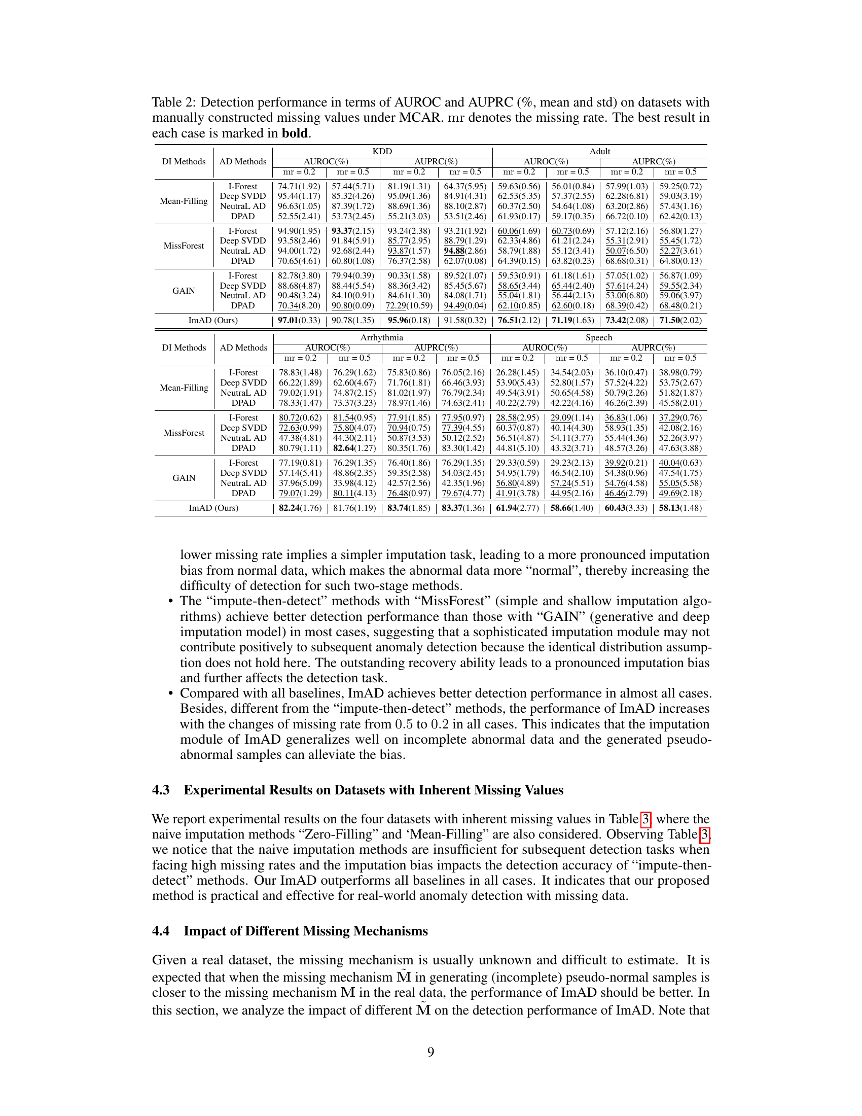
This table presents the results of anomaly detection experiments conducted on datasets with manually introduced missing values under the Missing Completely at Random (MCAR) mechanism. The performance of various anomaly detection methods is evaluated using two metrics: Area Under the Receiver Operating Characteristic curve (AUROC) and Area Under the Precision-Recall Curve (AUPRC). The table shows the mean and standard deviation for each method across multiple runs. The best-performing method for each dataset and missing rate is highlighted in bold. The results are broken down by imputation method (Mean-Filling, MissForest, GAIN) and anomaly detection method (I-Forest, Deep SVDD, NeutraL AD, DPAD). The table helps to compare the effectiveness of different imputation techniques in conjunction with various anomaly detection algorithms when dealing with missing data.
This table presents the results of anomaly detection experiments conducted on datasets with manually introduced missing values, under the Missing Completely at Random (MCAR) mechanism. The performance is evaluated using two metrics: Area Under the Receiver Operating Characteristic curve (AUROC) and Area Under the Precision-Recall curve (AUPRC). Different imputation methods (Mean-Filling, MissForest, GAIN) are combined with different anomaly detection methods (I-Forest, Deep SVDD, NeutraL AD, DPAD). The table shows the AUROC and AUPRC scores for each combination, along with their standard deviations. The best performance for each dataset and missing rate is highlighted in bold. The missing rate (mr) is either 0.2 or 0.5.

This table presents the performance of the ImAD model under different missing data mechanisms. It compares the Area Under the Receiver Operating Characteristic (AUROC) and Area Under the Precision-Recall Curve (AUPRC) scores achieved when using different missing mechanisms for both the normal training data and the generated pseudo-abnormal samples. The results demonstrate the robustness and sensitivity of the model to different missing data patterns, particularly when the assumed missingness mechanism used during training differs from the actual mechanism in the data. The datasets used are Titanic, MovieLens 1M, Bladder, Seq2-Heart, and Adult, with different missing mechanisms (MCAR, MAR, MNAR) applied to the data.

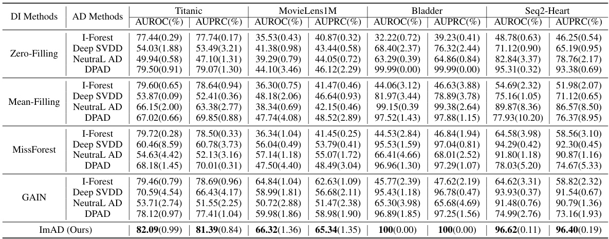
This table presents the performance of various anomaly detection methods on datasets with manually introduced missing values. The methods are evaluated using two metrics: AUROC (Area Under the Receiver Operating Characteristic curve) and AUPRC (Area Under the Precision-Recall curve). The missing values are introduced using the Missing Completely at Random (MCAR) mechanism. Results are presented as percentages with mean and standard deviation for different missing rates (mr). The best-performing method for each dataset and metric is highlighted in bold.

This table presents the performance of various anomaly detection methods on datasets with manually introduced missing values. The methods are compared using the Area Under the Receiver Operating Characteristic (AUROC) and Area Under the Precision-Recall Curve (AUPRC) metrics. The missing values are generated using the Missing Completely at Random (MCAR) mechanism, and different missing rates (mr) are tested. The table shows the average performance and standard deviations across multiple runs for each method, highlighting the best performing method for each dataset and missing rate.
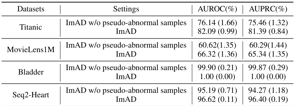
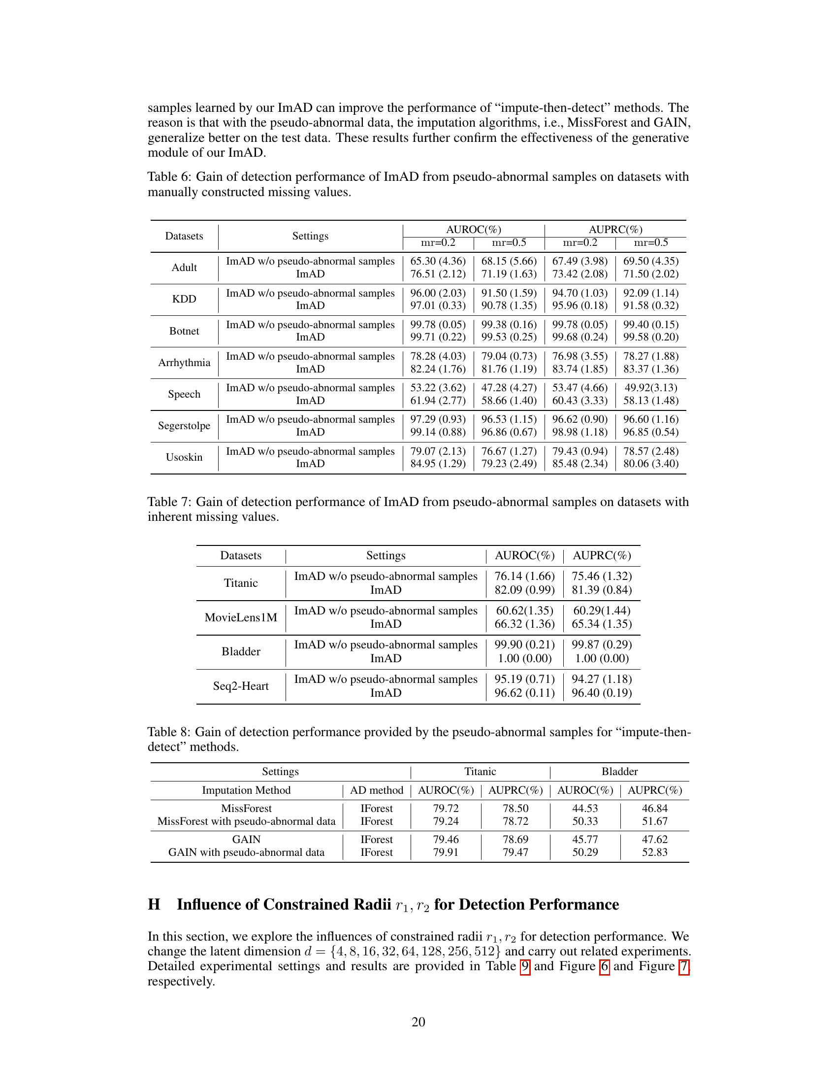
This table shows the improvement in AUROC and AUPRC achieved by ImAD when pseudo-abnormal samples are included in the training process, compared to when they are excluded. The results are presented for four datasets with inherent missing values (Titanic, MovieLens1M, Bladder, Seq2-Heart) and two settings (ImAD with and without pseudo-abnormal samples). The inclusion of pseudo-abnormal samples consistently leads to a notable performance increase.

This table presents the results of using pseudo-abnormal samples generated by ImAD to improve the performance of ‘impute-then-detect’ methods. It shows that adding pseudo-abnormal samples to the training data of MissForest and GAIN imputation methods leads to improvement in the AUROC and AUPRC scores of IForest anomaly detection, demonstrating that ImAD’s generated samples effectively mitigate the imputation bias.

This table presents the performance of various anomaly detection methods on datasets with manually introduced missing values. The methods are compared using two metrics: AUROC and AUPRC, with results shown for two missing rates (0.2 and 0.5). The best performing method for each scenario is highlighted in bold. The table helps to evaluate the effectiveness of different anomaly detection techniques in the presence of missing data, particularly focusing on the impact of imputation bias.
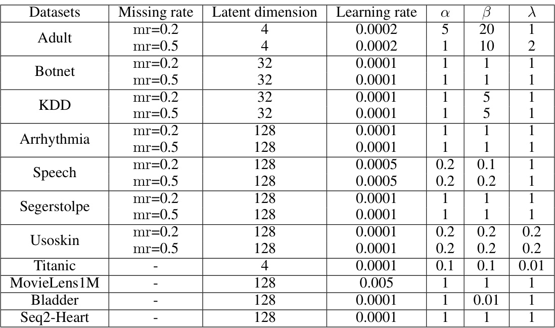
This table presents the characteristics of eleven datasets used in the experiments. For each dataset, it lists the field of study the data comes from, the number of features, the total number of instances, the number of normal and abnormal instances, the missing sample rate (percentage of samples with at least one missing value), and the missing entry rate (percentage of all entries that are missing). The datasets are categorized into those with inherent missing values and those with manually constructed missing values.

This table presents the performance of various anomaly detection methods on datasets with manually introduced missing values. The methods are categorized by the data imputation technique used (Mean-Filling, MissForest, GAIN) and the anomaly detection algorithm (IForest, Deep SVDD, NeutraL AD, DPAD). The results are shown for two different missing rates (0.2 and 0.5) and the best-performing method for each combination is highlighted. The table helps illustrate the effectiveness of different imputation strategies coupled with anomaly detection algorithms in handling missing data.
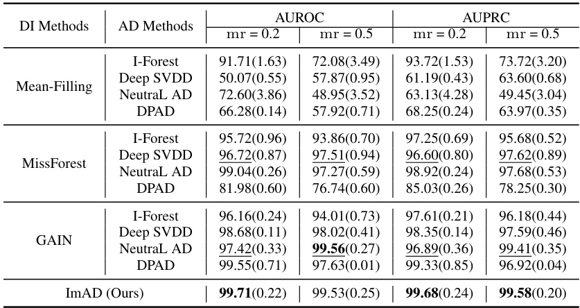
This table presents the performance comparison of different anomaly detection methods on datasets with manually introduced missing values under the Missing Completely At Random (MCAR) mechanism. The performance is evaluated using two metrics: AUROC (Area Under the Receiver Operating Characteristic curve) and AUPRC (Area Under the Precision-Recall curve). The table compares the performance of ImAD (the proposed method) against eight baseline methods that combine imputation techniques (Mean-Filling, MissForest, GAIN) with anomaly detection methods (Isolation Forest, Deep SVDD, NeuTraL AD, DPAD). The results are shown for two missing rates (mr = 0.2 and mr = 0.5). The best performing method for each dataset and metric is highlighted in bold.

This table presents the performance of different anomaly detection methods on datasets with manually introduced missing values. The methods are compared using two metrics: AUROC (Area Under the Receiver Operating Characteristic curve) and AUPRC (Area Under the Precision-Recall curve), both expressed as percentages. The performance is shown for two missing rates (mr = 0.2 and mr = 0.5) and is broken down by imputation method (Mean-Filling, MissForest, GAIN) and anomaly detection method (IForest, Deep SVDD, NeutraL AD, DPAD). The best performing method for each combination of dataset, missing rate, and metric is highlighted in bold.

This table presents the performance of different anomaly detection methods on the Adult dataset with missing values under the Missing At Random (MAR) mechanism. The performance is measured using AUROC and AUPRC, with the mean and standard deviation calculated across multiple runs. The table compares several imputation methods (Mean-Filling, MissForest, MissOT (MLP)) combined with several anomaly detection methods (I-Forest, Deep SVDD, NeutraL AD, DPAD). It also includes the results for the proposed ImAD method. The best-performing method in each scenario is highlighted in bold.
Full paper#


