TL;DR#
Single-task neural network training often results in non-unique solutions, hindering our understanding and control of the learning process. This paper investigates the properties of solutions to multi-task learning problems using shallow ReLU neural networks. Unlike single-task scenarios, the researchers demonstrate that multi-task learning problems exhibit nearly unique solutions, a finding that challenges common intuitions and existing theories in the field. This unexpected uniqueness is particularly interesting when dealing with a high number of tasks, making the problem well-approximated by a kernel method.
The study focuses on the behavior of the network’s solutions when trained on multiple diverse tasks. Through theoretical analysis and empirical observations, the authors show that the solutions for individual tasks are strikingly different from those obtained through single-task training. In the univariate case, they prove that the solution is almost always unique and equivalent to a minimum-norm interpolation problem in a reproducing kernel Hilbert space. Similar phenomena are observed in the multivariate case, showing the approximate equivalence to an l² minimization problem in a reproducing kernel Hilbert space, determined by the optimal neurons. This highlights the significant impact of multi-task learning on the regularization and behavior of neural networks.
Key Takeaways#
Why does it matter?#
This paper is crucial because it reveals a surprising connection between neural networks and kernel methods, particularly in multi-task learning. It challenges conventional wisdom and offers novel insights into the inductive bias of multi-task neural networks, potentially leading to improved training algorithms and a deeper understanding of their generalization capabilities. The uniqueness of solutions in multi-task settings is a significant advancement in the field. This work is also relevant to the current research trends on function spaces and representer theorems for neural networks.
Visual Insights#

🔼 The figure shows two different solutions obtained by training a ReLU neural network to interpolate the same dataset. Both solutions minimize the sum of squared weights and the second-order total variation of the interpolating function, highlighting the non-uniqueness of solutions in single-task neural network training. The solutions differ significantly in their shape, demonstrating that even though they are both optimal solutions, one of them is visually much more appealing.
read the caption
Figure 1: Two solutions to ReLU neural network interpolation (blue) of training data (red). The functions on the left and right both interpolate the data and both are global minimizers of (2) and (3), and minimize the second-order total variation of the interpolation function Parhi and Nowak (2021). In fact, all convex combinations of the two solutions above are also global solutions to both training problems.
In-depth insights#
Multi-task Uniqueness#
The concept of ‘Multi-task Uniqueness’ in the context of neural network training is a significant departure from traditional single-task learning paradigms. In single-task learning, the solution is often non-unique, meaning multiple network configurations can achieve similar performance on a given dataset. Multi-task learning, however, can introduce a uniqueness constraint. By training a shared network on multiple tasks simultaneously, certain tasks might impose sufficient constraints on the parameter space to eliminate the multiplicity of solutions. The analysis of conditions under which this uniqueness emerges is crucial, and could involve studying the properties of the objective function, the nature of the tasks themselves, and the network architecture. A deeper understanding of this could pave the way for improving generalization performance by reducing overfitting, as well as developing more efficient training algorithms. The implications are profound, suggesting that the very process of multi-task learning fundamentally alters the inductive biases of neural networks. This insight could be exploited to enhance the robustness of models and improve performance in scenarios where data is limited or noisy.
Kernel Equivalence#
The concept of “Kernel Equivalence” in the context of multi-task neural network learning is a significant finding. It suggests that under specific conditions (e.g., a large number of diverse tasks and minimal sum-of-squared weights regularization), the solutions learned by a neural network for individual tasks closely approximate those obtained by kernel methods. This bridges the gap between neural networks and kernel methods, revealing an unexpected connection. The implications are profound: it suggests that the inductive bias of multi-task learning, even with unrelated tasks, can be characterized as promoting solutions that lie within a specific Reproducing Kernel Hilbert Space (RKHS), leading to potential benefits in generalization and robustness. The almost always unique nature of these solutions, unlike single-task learning, is another key aspect of this “Kernel Equivalence.” This uniqueness implies improved predictability and control over the function learned, potentially resolving issues of non-uniqueness and sensitivity inherent in single-task neural network training. Further research should explore the precise conditions under which this equivalence holds and its implications for various machine learning applications.
Multivariate Insights#
Extending the single-task, univariate analysis to the multivariate setting presents a significant challenge. The non-convex nature of the optimization problem is exacerbated by the increased dimensionality, making it far more difficult to guarantee uniqueness of solutions. The authors hypothesize that with a large number of diverse tasks, the solutions for each individual task will approach minimum-norm solutions within a Reproducing Kernel Hilbert Space (RKHS), determined by the optimal neurons. This implies a shift from the non-Hilbertian Banach space norms observed in the single-task scenario to a more regularized Hilbert space setting in the multi-task case. This transition suggests that multi-task learning might implicitly impose a form of regularization, effectively resolving the non-uniqueness issue observed in single-task scenarios by converging to well-behaved solutions within a specific RKHS. Empirical evidence is presented to support this claim, although rigorous mathematical proof in the multivariate case remains an open problem. The observed phenomenon has significant implications, suggesting that multi-task learning could act as a powerful implicit regularizer, leading to improved generalization and robustness compared to traditional single-task training methodologies. Further investigation into the characteristics of the resulting RKHS, including its dependence on the nature and diversity of the tasks, is crucial for a deeper understanding of this phenomenon.
Limitations and Future#
The research primarily focuses on theoretical analysis of multi-task learning in shallow ReLU networks, thus limiting its direct applicability to real-world scenarios with complex architectures and noisy data. The univariate analysis, while providing strong theoretical results, lacks generalization to high-dimensional settings common in practice. Although empirical evidence is given, a more thorough experimental evaluation with diverse, large-scale datasets is needed to validate the findings. Future work could explore extending the analysis to deeper networks and other activation functions, improving the empirical validation with more extensive experiments, and investigating the impact of task similarity and data distribution on the uniqueness of solutions. Furthermore, exploring the application of these findings to improve existing multi-task learning algorithms and addressing practical challenges like computational complexity and hyperparameter tuning would greatly enhance the practical impact of the research. Investigating alternative regularization schemes could also provide additional insights into the inductive bias of multi-task learning.
Experimental Setup#
A hypothetical ‘Experimental Setup’ section for this research paper would detail the specifics of the numerical experiments used to validate the theoretical findings. This would include a precise description of the datasets employed, specifying their size, dimensionality, and generation method (e.g., synthetic or real-world), particularly noting whether the datasets were designed to satisfy or violate specific conditions (like aligned vectors) impacting solution uniqueness. The choice of neural network architecture (including width, activation function, and number of layers) along with the optimization algorithm (e.g., Adam, gradient descent) and hyperparameters used must be meticulously documented. The choice of loss function (e.g., mean squared error), regularization techniques (e.g., weight decay), and the methods for evaluating results (e.g., error metrics) are critical elements. The description must emphasize the reproducibility of the experiments, outlining the procedures to ensure that the reported results can be obtained by other researchers using the same settings and methodology. It should also clarify the number of trials performed for each experiment and how randomness (e.g., in initialization) was handled to ensure reliable and unbiased results. The section would conclude by highlighting any limitations or potential biases inherent in the experimental design, explaining why these limitations may not affect the conclusions reached.
More visual insights#
More on figures

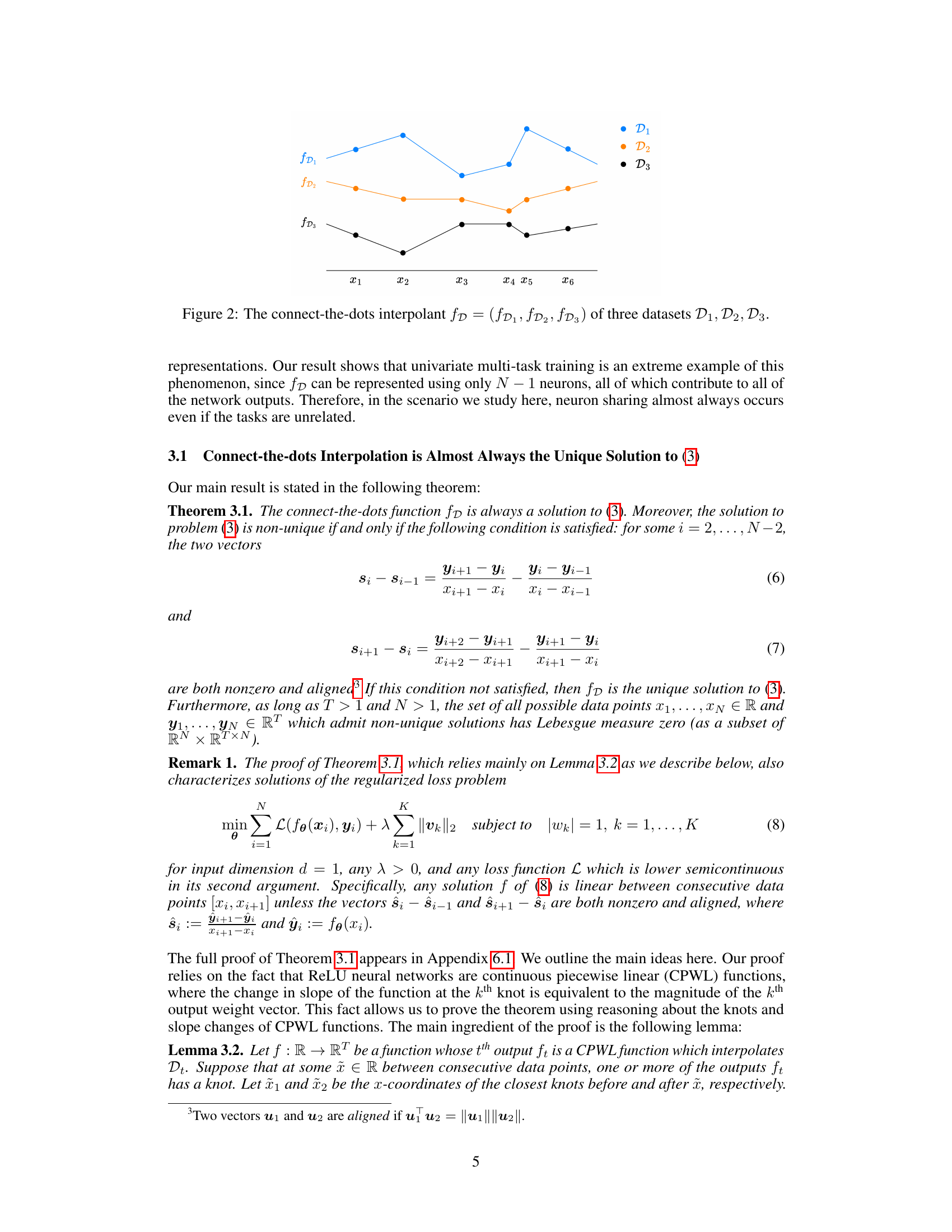
🔼 This figure shows an example of the connect-the-dots interpolant for three different datasets. Each dataset has its own set of data points which are connected by a straight line. This creates a piecewise linear function for each dataset. The figure illustrates that the connect-the-dots interpolant is a simple, yet effective, way to approximate a function that fits the given data. This method is important in the context of the paper as it relates to finding unique solutions for multi-task neural network training problems.
read the caption
Figure 2: The connect-the-dots interpolant fD = (fD1, fD2, fD3) of three datasets D1, D2, D3.
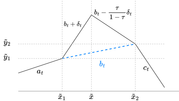
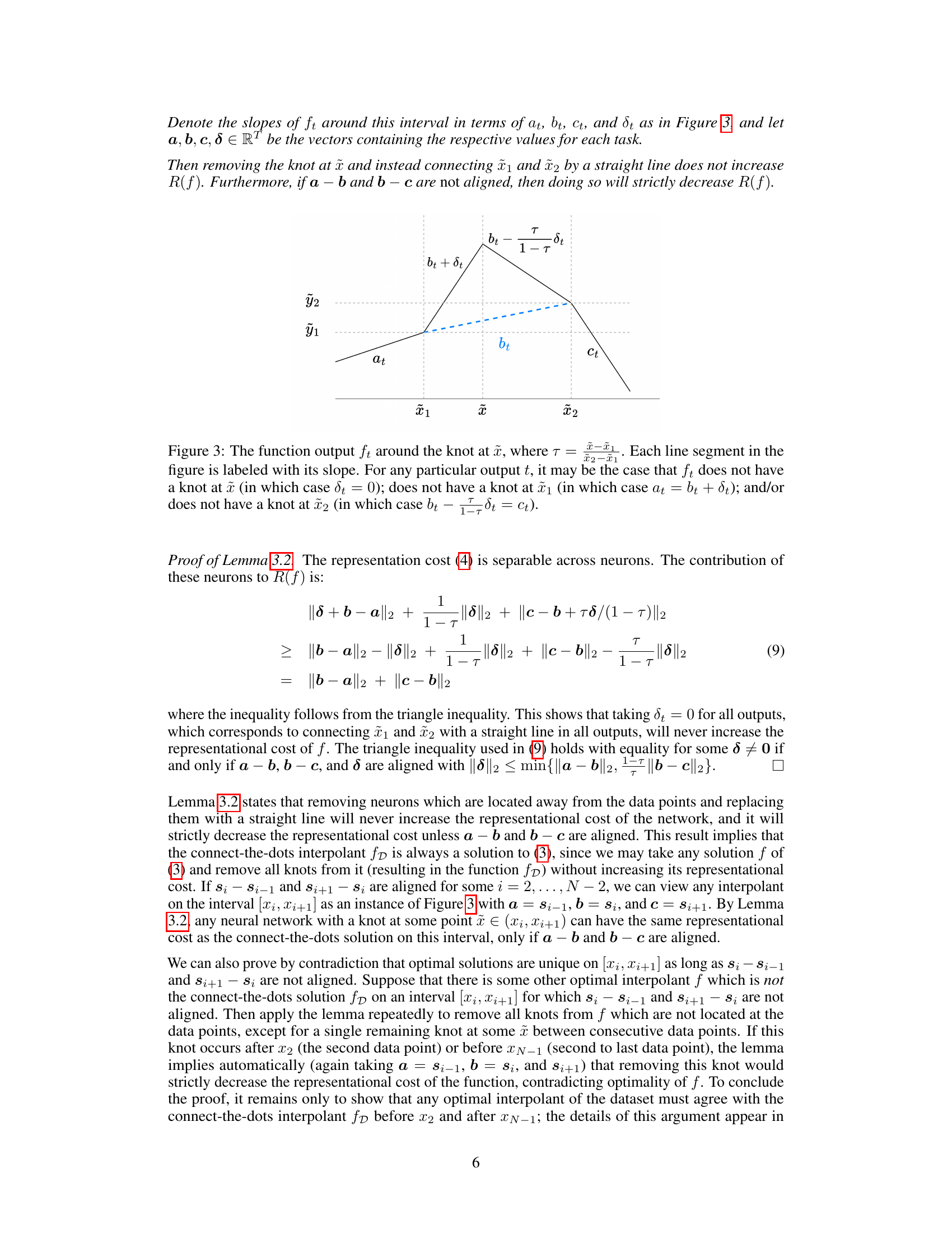
🔼 This figure illustrates the function output (ft) around a knot at point x. It shows how the slopes (at, bt, ct, dt) change around the knot and how the removal of the knot affects the representation cost. The figure clarifies that the absence of a knot at points x1 or x2 results in specific equalities among the slopes.
read the caption
Figure 3: The function output ft around the knot at x, where τ = x−x1/x2−x1. Each line segment in the figure is labeled with its slope. For any particular output t, it may be the case that ft does not have a knot at x (in which case dt = 0); does not have a knot at x1 (in which case at = bt + τδt); and/or does not have a knot at x2 (in which case bt − (1−τ)δt = ct).
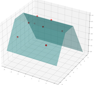
🔼 This figure compares single-task and multi-task ReLU neural network interpolation in 2D. Single-task solutions show multiple global minimizers, while multi-task solutions are nearly identical and close to the RKHS approximation.
read the caption
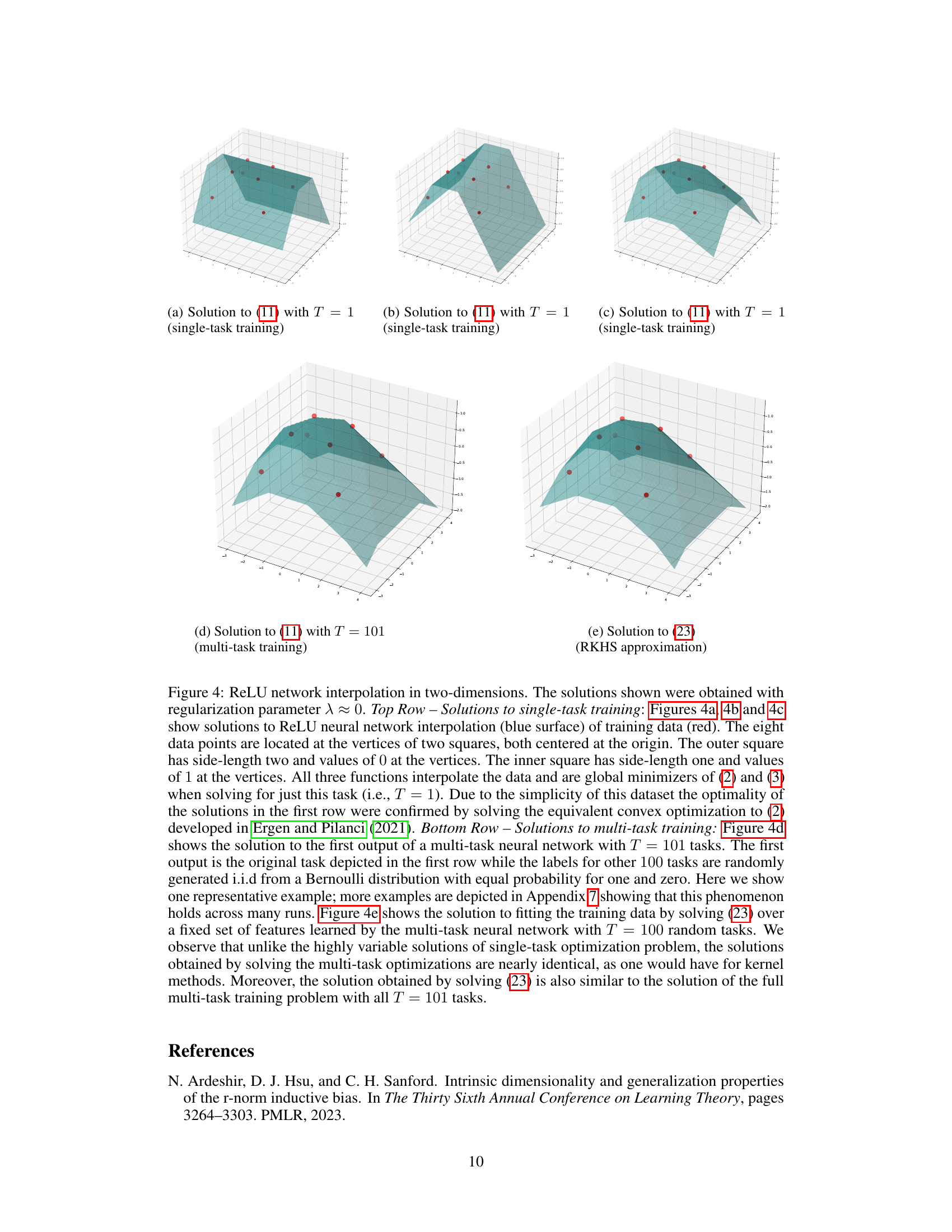
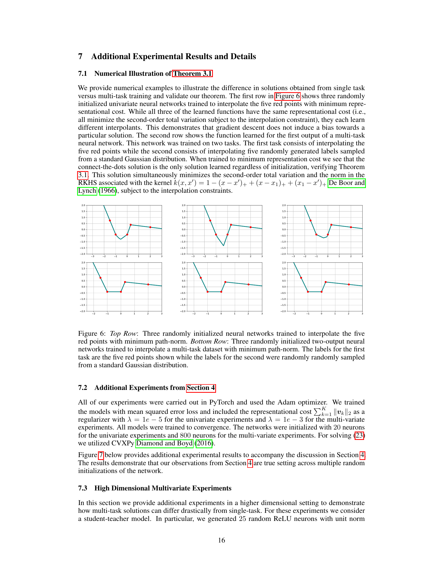
Figure 4: ReLU network interpolation in two-dimensions. The solutions shown were obtained with regularization parameter λ ≈ 0. Top Row – Solutions to single-task training: Figures 4a, 4b and 4c show solutions to ReLU neural network interpolation (blue surface) of training data (red). The eight data points are located at the vertices of two squares, both centered at the origin. The outer square has side-length two and values of 0 at the vertices. The inner square has side-length one and values of 1 at the vertices. All three functions interpolate the data and are global minimizers of (2) and (3) when solving for just this task (i.e., T = 1). Due to the simplicity of this dataset the optimality of the solutions in the first row were confirmed by solving the equivalent convex optimization to (2) developed in Ergen and Pilanci (2021). Bottom Row – Solutions to multi-task training: Figure 4d shows the solution to the first output of a multi-task neural network with T = 101 tasks. The first output is the original task depicted in the first row while the labels for other 100 tasks are randomly generated i.i.d from a Bernoulli distribution with equal probability for one and zero. Here we show one representative example; more examples are depicted in Appendix 7 showing that this phenomenon holds across many runs. Figure 4e shows the solution to fitting the training data by solving (23) over a fixed set of features learned by the multi-task neural network with T = 100 random tasks. We observe that unlike the highly variable solutions of single-task optimization problem, the solutions obtained by solving multi-task optimizations are nearly identical, as one would have for kernel methods. Moreover, the solution obtained by solving (23) is also similar to the solution of the full multi-task training problem with all T = 101 tasks.
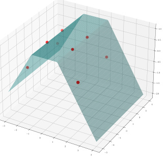
🔼 This figure compares solutions obtained from single-task and multi-task training of ReLU neural networks. Single-task training yields multiple solutions, while multi-task training with many diverse tasks yields a unique solution that closely resembles the solution to a kernel method.
read the caption
Figure 4: ReLU network interpolation in two-dimensions. The solutions shown were obtained with regularization parameter λ ≈ 0. Top Row – Solutions to single-task training: Figures 4a, 4b and 4c show solutions to ReLU neural network interpolation (blue surface) of training data (red). The eight data points are located at the vertices of two squares, both centered at the origin. The outer square has side-length two and values of 0 at the vertices. The inner square has side-length one and values of 1 at the vertices. All three functions interpolate the data and are global minimizers of (2) and (3) when solving for just this task (i.e., T = 1). Due to the simplicity of this dataset the optimality of the solutions in the first row were confirmed by solving the equivalent convex optimization to (2) developed in Ergen and Pilanci (2021). Bottom Row – Solutions to multi-task training: Figure 4d shows the solution to the first output of a multi-task neural network with T = 101 tasks. The first output is the original task depicted in the first row while the labels for other 100 tasks are randomly generated i.i.d from a Bernoulli distribution with equal probability for one and zero. Here we show one representative example; more examples are depicted in Appendix 7 showing that this phenomenon holds across many runs. Figure 4e shows the solution to fitting the training data by solving (23) over a fixed set of features learned by the multi-task neural network with T = 100 random tasks. We observe that unlike the highly variable solutions of single-task optimization problem, the solutions obtained by solving multi-task optimizations are nearly identical, as one would have for kernel methods. Moreover, the solution obtained by solving (23) is also similar to the solution of the full multi-task training problem with all T = 101 tasks.

🔼 This figure compares single-task and multi-task ReLU neural network interpolation results on a simple 2D dataset. Single-task solutions show non-uniqueness, while multi-task learning with many tasks produces a nearly unique, smooth solution similar to a kernel method.
read the caption
Figure 4: ReLU network interpolation in two-dimensions. The solutions shown were obtained with regularization parameter λ ≈ 0. Top Row – Solutions to single-task training: Figures 4a, 4b and 4c show solutions to ReLU neural network interpolation (blue surface) of training data (red). The eight data points are located at the vertices of two squares, both centered at the origin. The outer square has side-length two and values of 0 at the vertices. The inner square has side-length one and values of 1 at the vertices. All three functions interpolate the data and are global minimizers of (2) and (3) when solving for just this task (i.e., T = 1). Due to the simplicity of this dataset the optimality of the solutions in the first row were confirmed by solving the equivalent convex optimization to (2) developed in Ergen and Pilanci (2021). Bottom Row – Solutions to multi-task training: Figure 4d shows the solution to the first output of a multi-task neural network with T = 101 tasks. The first output is the original task depicted in the first row while the labels for other 100 tasks are randomly generated i.i.d from a Bernoulli distribution with equal probability for one and zero. Here we show one representative example; more examples are depicted in Appendix 7 showing that this phenomenon holds across many runs. Figure 4e shows the solution to fitting the training data by solving (23) over a fixed set of features learned by the multi-task neural network with T = 100 random tasks. We observe that unlike the highly variable solutions of single-task optimization problem, the solutions obtained by solving multi-task optimizations are nearly identical, as one would have for kernel methods. Moreover, the solution obtained by solving (23) is also similar to the solution of the full multi-task training problem with all T = 101 tasks.

🔼 This figure compares single-task and multi-task solutions for a 2D interpolation problem. Single-task solutions show non-uniqueness, while multi-task solutions are almost always unique and approximate the solution to a kernel method.
read the caption
Figure 4: ReLU network interpolation in two-dimensions. The solutions shown were obtained with regularization parameter λ ≈ 0. Top Row – Solutions to single-task training: Figures 4a, 4b and 4c show solutions to ReLU neural network interpolation (blue surface) of training data (red). The eight data points are located at the vertices of two squares, both centered at the origin. The outer square has side-length two and values of 0 at the vertices. The inner square has side-length one and values of 1 at the vertices. All three functions interpolate the data and are global minimizers of (2) and (3) when solving for just this task (i.e., T = 1). Due to the simplicity of this dataset the optimality of the solutions in the first row were confirmed by solving the equivalent convex optimization to (2) developed in Ergen and Pilanci (2021). Bottom Row – Solutions to multi-task training: Figure 4d shows the solution to the first output of a multi-task neural network with T = 101 tasks. The first output is the original task depicted in the first row while the labels for other 100 tasks are randomly generated i.i.d from a Bernoulli distribution with equal probability for one and zero. Here we show one representative example; more examples are depicted in Appendix 7 showing that this phenomenon holds across many runs. Figure 4e shows the solution to fitting the training data by solving (23) over a fixed set of features learned by the multi-task neural network with T = 100 random tasks. We observe that unlike the highly variable solutions of single-task optimization problem, the solutions obtained by solving the multi-task optimizations are nearly identical, as one would have for kernel methods. Moreover, the solution obtained by solving (23) is also similar to the solution of the full multi-task training problem with all T = 101 tasks.

🔼 This figure compares single-task and multi-task ReLU neural network solutions for a simple 2D interpolation problem. Single-task solutions exhibit high variability, while multi-task solutions (with many diverse tasks) converge to a nearly identical, smooth solution resembling a kernel method.
read the caption
Figure 4: ReLU network interpolation in two-dimensions. The solutions shown were obtained with regularization parameter λ ≈ 0. Top Row – Solutions to single-task training: Figures 4a, 4b and 4c show solutions to ReLU neural network interpolation (blue surface) of training data (red). The eight data points are located at the vertices of two squares, both centered at the origin. The outer square has side-length two and values of 0 at the vertices. The inner square has side-length one and values of 1 at the vertices. All three functions interpolate the data and are global minimizers of (2) and (3) when solving for just this task (i.e., T = 1). Due to the simplicity of this dataset the optimality of the solutions in the first row were confirmed by solving the equivalent convex optimization to (2) developed in Ergen and Pilanci (2021). Bottom Row – Solutions to multi-task training: Figure 4d shows the solution to the first output of a multi-task neural network with T = 101 tasks. The first output is the original task depicted in the first row while the labels for other 100 tasks are randomly generated i.i.d from a Bernoulli distribution with equal probability for one and zero. Here we show one representative example; more examples are depicted in Appendix 7 showing that this phenomenon holds across many runs. Figure 4e shows the solution to fitting the training data by solving (23) over a fixed set of features learned by the multi-task neural network with T = 100 random tasks. We observe that unlike the highly variable solutions of single-task optimization problem, the solutions obtained by solving multi-task optimizations are nearly identical, as one would have for kernel methods. Moreover, the solution obtained by solving (23) is also similar to the solution of the full multi-task training problem with all T = 101 tasks.
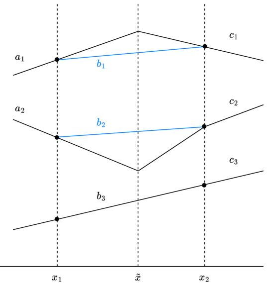
🔼 This figure shows a piecewise linear function with a knot at point x. It illustrates how the slopes of the function (at, bt, ct, dt) change around the knot, and how the removal of the knot affects the representational cost of the function.
read the caption
Figure 3: The function output ft around the knot at x, where τ = (x2 − x)/(x2 − x1). Each line segment in the figure is labeled with its slope. For any particular output t, it may be the case that ft does not have a knot at x (in which case dt = 0); does not have a knot at x1 (in which case at = bt + τδt); and/or does not have a knot at x2 (in which case bt − (1 − τ)δt = ct).
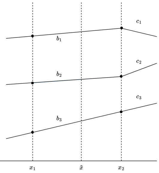
🔼 This figure shows two plots that illustrate the concept behind Lemma 3.2. The left plot shows a function g with a knot at some point x between two data points x1 and x2. The right plot shows the connect-the-dots interpolant fD, which is a piecewise linear function connecting the data points without any extra knots. The caption highlights that the representational cost R(g) of the function with the knot is strictly greater than the representational cost R(fD) of the connect-the-dots interpolant.
read the caption
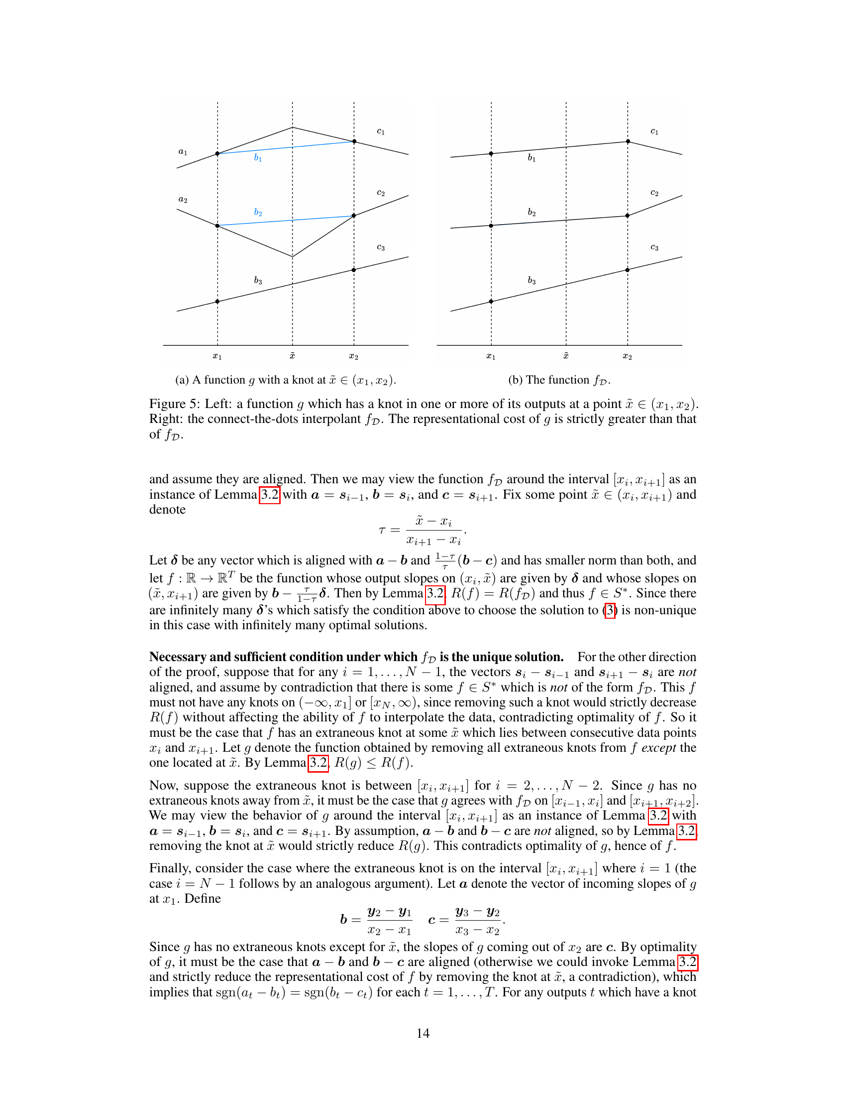
Figure 5: Left: a function g which has a knot in one or more of its outputs at a point x ∈ (x1, x2). Right: the connect-the-dots interpolant fD. The representational cost of g is strictly greater than that of fD.
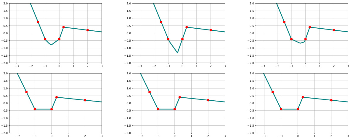
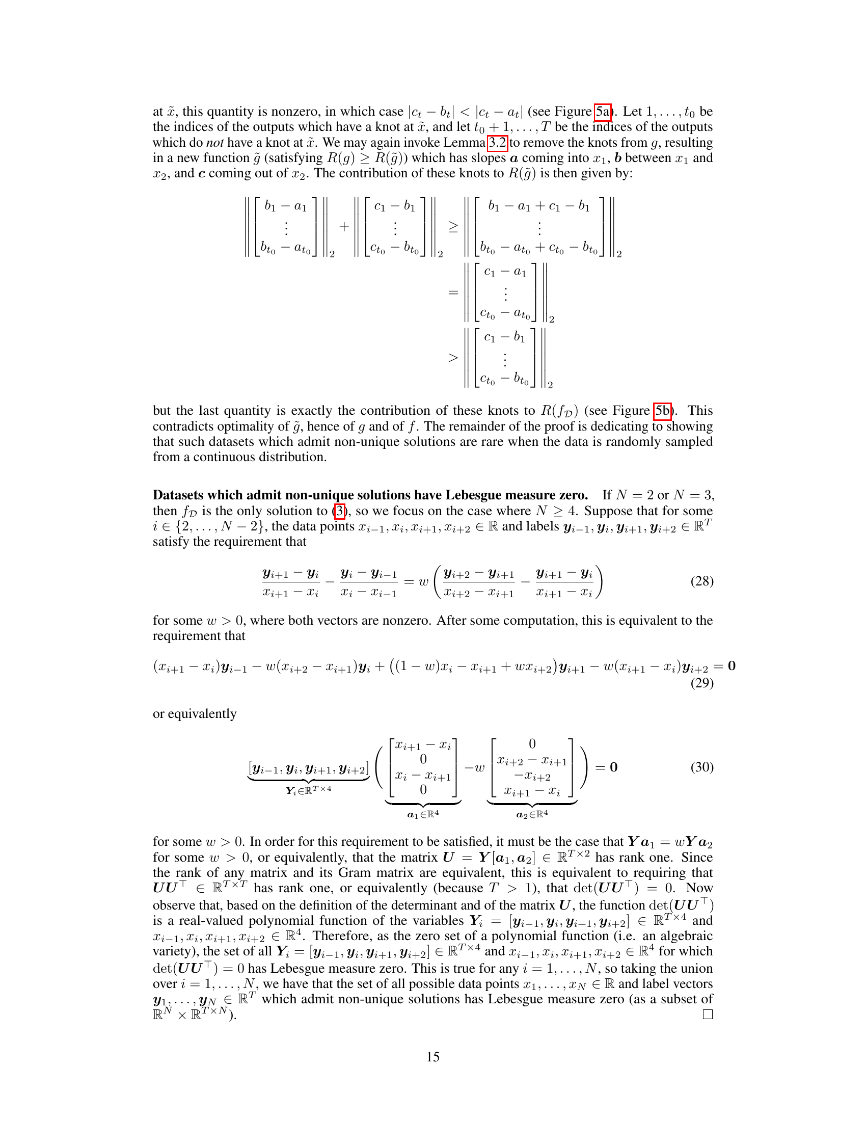
🔼 This figure demonstrates the difference between solutions obtained from single-task vs. multi-task training. The top row shows three randomly initialized neural networks, each trained to interpolate five data points (red dots) with minimum representational cost, highlighting non-uniqueness in single-task solutions. The bottom row presents the solution obtained for the first output of a multi-task network (with the same five red points as the first task, and a second task with labels randomly sampled from a standard Gaussian distribution). This illustrates the uniqueness and connect-the-dots nature of multi-task solutions.
read the caption
Figure 6: Top Row: Three randomly initialized neural networks trained to interpolate the five red points with minimum path-norm. Bottom Row: Three randomly initialized two-output neural networks trained to interpolate a multi-task dataset with minimum path-norm. The labels for the first task are the five red points shown while the labels for the second were randomly randomly sampled from a standard Gaussian distribution.

🔼 This figure compares single-task and multi-task solutions to ReLU neural network interpolation problems in 2D. The single-task solutions show significant variability, while the multi-task solution is unique and similar to the solution of a kernel method.
read the caption
Figure 4: ReLU network interpolation in two-dimensions. The solutions shown were obtained with regularization parameter λ ≈ 0. Top Row – Solutions to single-task training: Figures 4a, 4b and 4c show solutions to ReLU neural network interpolation (blue surface) of training data (red). The eight data points are located at the vertices of two squares, both centered at the origin. The outer square has side-length two and values of 0 at the vertices. The inner square has side-length one and values of 1 at the vertices. All three functions interpolate the data and are global minimizers of (2) and (3) when solving for just this task (i.e., T = 1). Due to the simplicity of this dataset the optimality of the solutions in the first row were confirmed by solving the equivalent convex optimization to (2) developed in Ergen and Pilanci (2021). Bottom Row – Solutions to multi-task training: Figure 4d shows the solution to the first output of a multi-task neural network with T = 101 tasks. The first output is the original task depicted in the first row while the labels for other 100 tasks are randomly generated i.i.d from a Bernoulli distribution with equal probability for one and zero. Here we show one representative example; more examples are depicted in Appendix 7 showing that this phenomenon holds across many runs. Figure 4e shows the solution to fitting the training data by solving (23) over a fixed set of features learned by the multi-task neural network with T = 100 random tasks. We observe that unlike the highly variable solutions of single-task optimization problem, the solutions obtained by solving (23) are nearly identical, as one would have for kernel methods. Moreover, the solution obtained by solving (23) is also similar to the solution of the full multi-task training problem with all T = 101 tasks.

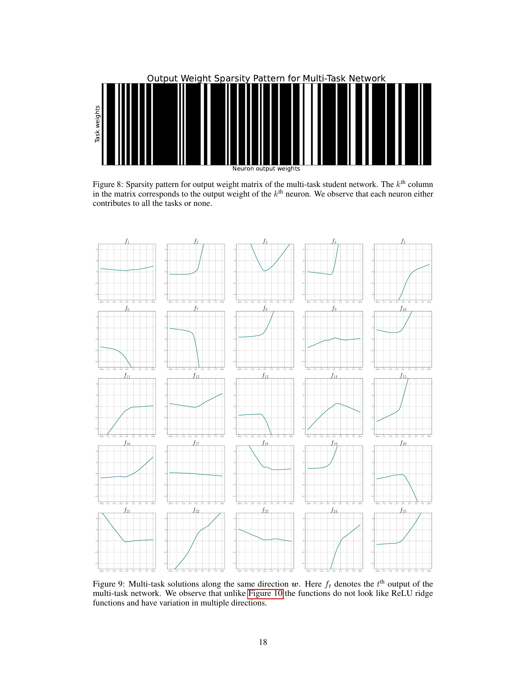
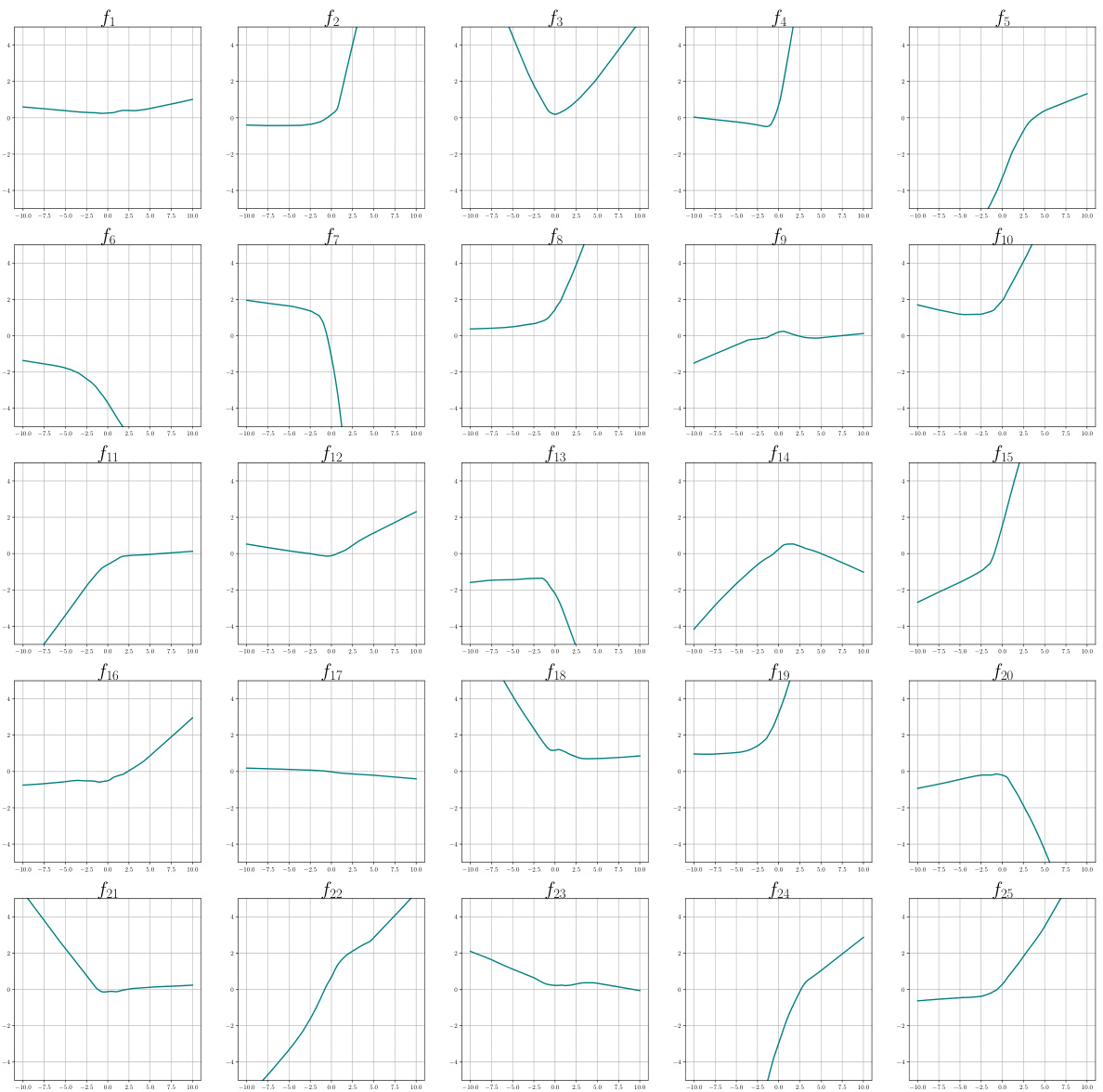
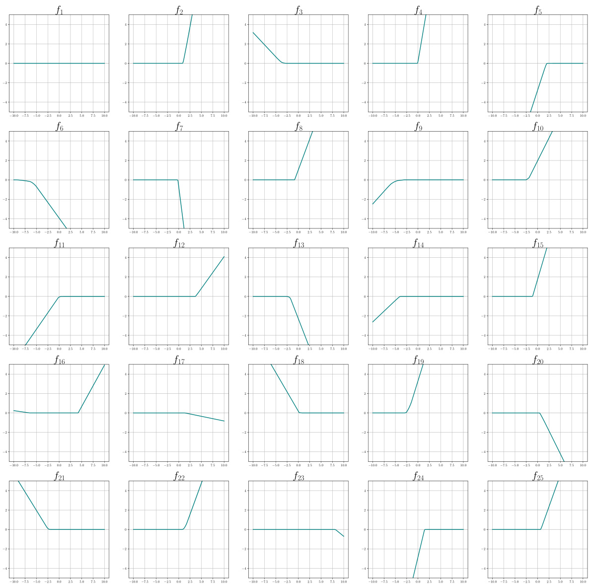
🔼 This figure shows the sparsity pattern of the output weight matrix for a multi-task neural network. Each column represents a neuron, and each row represents a task. A black square indicates that the neuron contributes to that task, while a white square indicates that it does not. The pattern shows that most neurons either contribute to all tasks or to none, illustrating neuron sharing behavior in multi-task learning.
read the caption
Figure 8: Sparsity pattern for output weight matrix of the multi-task student network. The kth column in the matrix corresponds to the output weight of the kth neuron. We observe that each neuron either contributes to all the tasks or none.
🔼 This figure compares single-task and multi-task ReLU neural network interpolations in 2D. Single-task solutions show non-uniqueness, while multi-task solutions (with many tasks) converge to a unique solution resembling a kernel method solution.
read the caption
Figure 4: ReLU network interpolation in two-dimensions. The solutions shown were obtained with regularization parameter λ ≈ 0. Top Row – Solutions to single-task training: Figures 4a, 4b and 4c show solutions to ReLU neural network interpolation (blue surface) of training data (red). The eight data points are located at the vertices of two squares, both centered at the origin. The outer square has side-length two and values of 0 at the vertices. The inner square has side-length one and values of 1 at the vertices. All three functions interpolate the data and are global minimizers of (2) and (3) when solving for just this task (i.e., T = 1). Due to the simplicity of this dataset the optimality of the solutions in the first row were confirmed by solving the equivalent convex optimization to (2) developed in Ergen and Pilanci (2021). Bottom Row – Solutions to multi-task training: Figure 4d shows the solution to the first output of a multi-task neural network with T = 101 tasks. The first output is the original task depicted in the first row while the labels for other 100 tasks are randomly generated i.i.d from a Bernoulli distribution with equal probability for one and zero. Here we show one representative example; more examples are depicted in Appendix 7 showing that this phenomenon holds across many runs. Figure 4e shows the solution to fitting the training data by solving (23) over a fixed set of features learned by the multi-task neural network with T = 100 random tasks. We observe that unlike the highly variable solutions of single-task optimization problem, the solutions obtained by solving multi-task optimizations are nearly identical, as one would have for kernel methods. Moreover, the solution obtained by solving (23) is also similar to the solution of the full multi-task training problem with all T = 101 tasks.
🔼 This figure compares single-task and multi-task solutions for a 2D interpolation problem. Single-task solutions show non-uniqueness, while multi-task solutions are nearly identical and closely approximate the RKHS solution.
read the caption
Figure 4: ReLU network interpolation in two-dimensions. The solutions shown were obtained with regularization parameter λ ≈ 0. Top Row – Solutions to single-task training: Figures 4a, 4b and 4c show solutions to ReLU neural network interpolation (blue surface) of training data (red). The eight data points are located at the vertices of two squares, both centered at the origin. The outer square has side-length two and values of 0 at the vertices. The inner square has side-length one and values of 1 at the vertices. All three functions interpolate the data and are global minimizers of (2) and (3) when solving for just this task (i.e., T = 1). Due to the simplicity of this dataset the optimality of the solutions in the first row were confirmed by solving the equivalent convex optimization to (2) developed in Ergen and Pilanci (2021). Bottom Row – Solutions to multi-task training: Figure 4d shows the solution to the first output of a multi-task neural network with T = 101 tasks. The first output is the original task depicted in the first row while the labels for other 100 tasks are randomly generated i.i.d from a Bernoulli distribution with equal probability for one and zero. Here we show one representative example; more examples are depicted in Appendix 7 showing that this phenomenon holds across many runs. Figure 4e shows the solution to fitting the training data by solving (23) over a fixed set of features learned by the multi-task neural network with T = 100 random tasks. We observe that unlike the highly variable solutions of single-task optimization problem, the solutions obtained by solving the multi-task optimizations are nearly identical, as one would have for kernel methods. Moreover, the solution obtained by solving (23) is also similar to the solution of the full multi-task training problem with all T = 101 tasks.
Full paper#
