TL;DR#
Current DNA tokenization methods borrow from NLP, ignoring DNA’s unique characteristics (discontinuous, overlapping, ambiguous segments), leading to suboptimal results. The optimal approach remains largely unexplored, and effective strategies may not be intuitively understood by researchers.
MxDNA uniquely addresses this by employing a sparse Mixture of Convolution Experts coupled with deformable convolutions. The model learns an effective tokenization strategy through gradient descent. MxDNA demonstrates superior performance on benchmark datasets using less pretraining data and time. Notably, it learns unique tokenization strategies and captures genomic functionalities. This novel framework offers broad applications in various domains and yields profound insights into DNA sequence analysis.
Key Takeaways#
Why does it matter?#
This paper is crucial for researchers in genomics and NLP because it introduces a novel approach to DNA sequence tokenization that outperforms existing methods and offers new biological insights. This research addresses the limitations of current methods, which are often unsuitable for DNA sequences, by allowing the model to autonomously learn an effective tokenization strategy. The findings have broad applications in various genomic research areas and could potentially revolutionize how we analyze DNA data. This opens new avenues for improving foundation models’ performance in genomics.
Visual Insights#
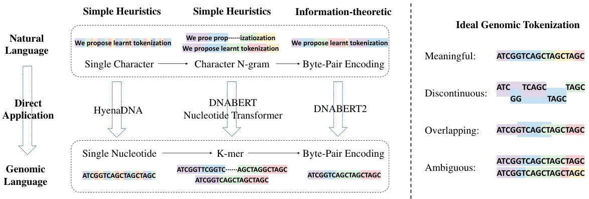
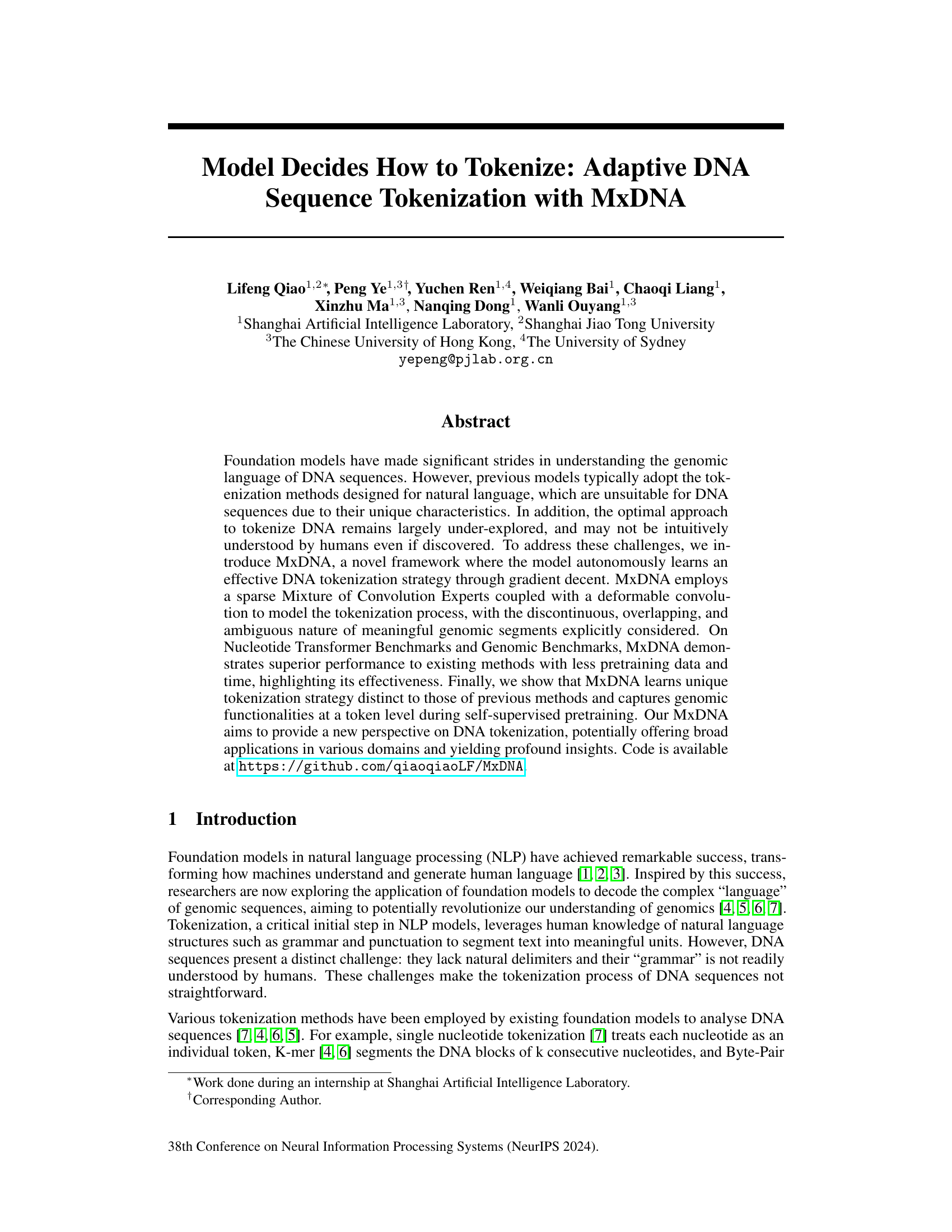
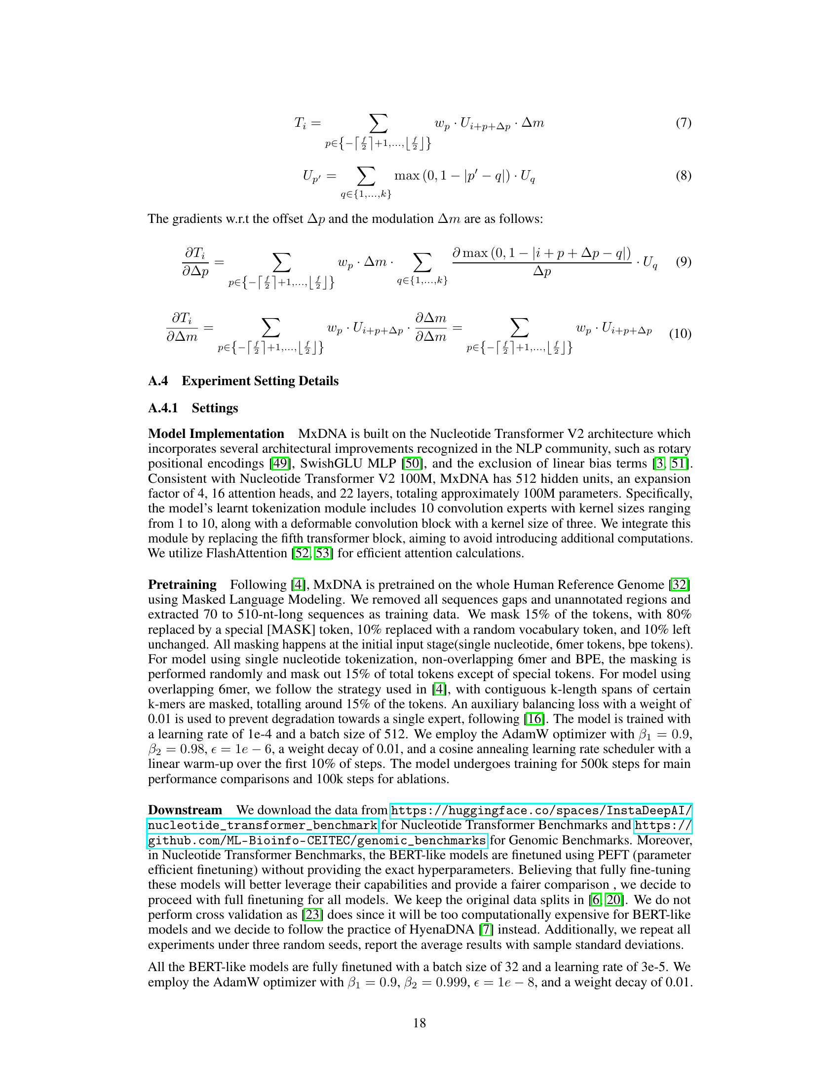
🔼 This figure illustrates the evolution of tokenization methods from simple heuristics used in natural language processing (NLP) to more sophisticated techniques applied to genomic sequences. The left side shows how NLP methods like single character, character N-grams, and Byte Pair Encoding (BPE) have been directly applied to DNA, but these methods have limitations due to the unique characteristics of DNA sequences. The right side presents the ideal properties of a genomic tokenizer as meaningful segments, allowing for discontinuous, overlapping, and ambiguous tokens, reflecting the complex and varied nature of DNA. The figure highlights that MxDNA aims to achieve these ideal properties for genomic sequence tokenization.
read the caption
Figure 1: Evolution of tokenization and Ideal Properties. Left: The progression from basic tokenization methods to more sophisticated techniques, with the direct but unsuitable applications from natural language to genomic language. Right: the ideal tokenization properties for genomics—Meaningful, Discontinuous, Overlapping, and Ambiguous-outlined in [8], which our MxDNA aims to achieve.
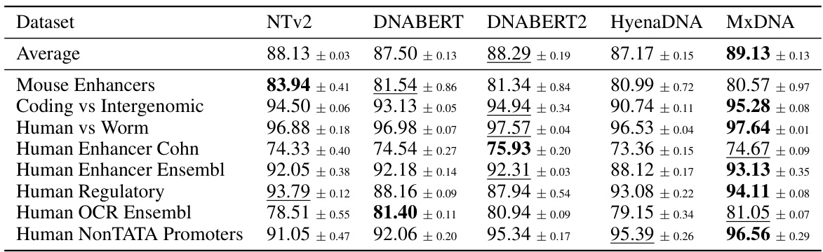
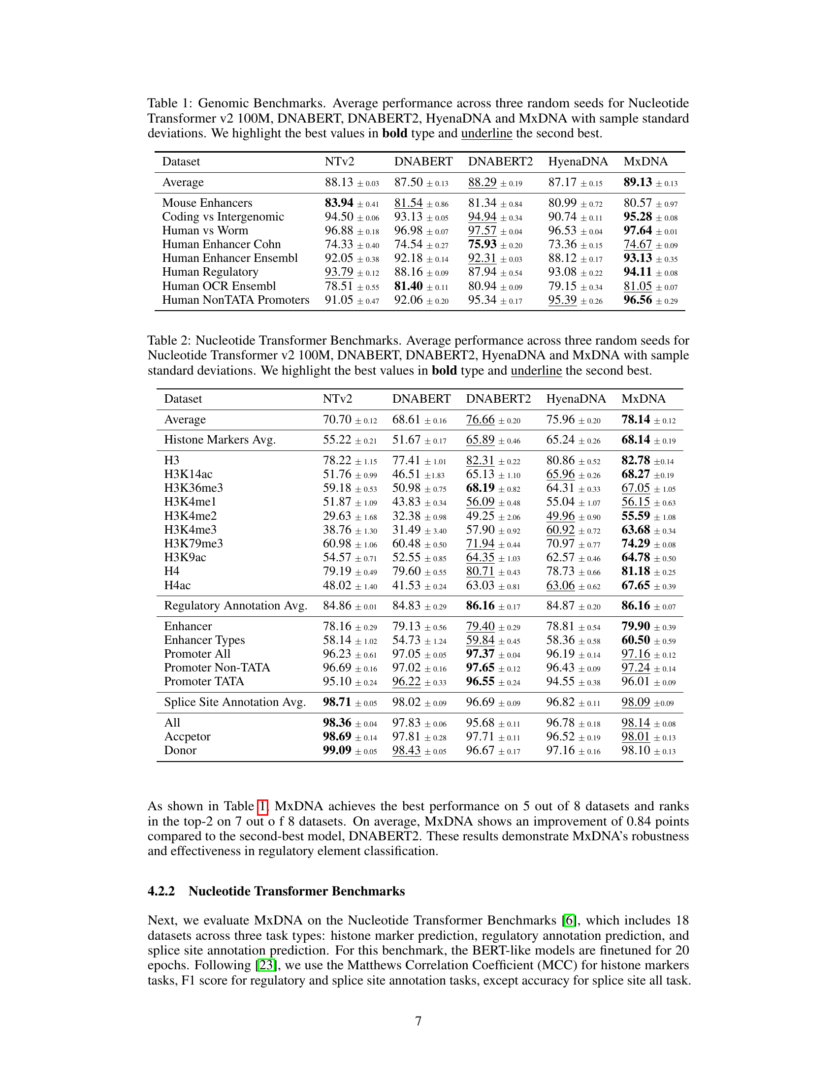
🔼 This table presents the average performance and standard deviation across three random seeds for five different models (Nucleotide Transformer v2 100M, DNABERT, DNABERT2, HyenaDNA, and MxDNA) on eight genomic datasets. The best performance for each dataset is highlighted in bold, and the second-best is underlined. The table allows for a comparison of the different models’ performance on various genomic tasks.
read the caption
Table 1: Genomic Benchmarks. Average performance across three random seeds for Nucleotide Transformer v2 100M, DNABERT, DNABERT2, HyenaDNA and MxDNA with sample standard deviations. We highlight the best values in bold type and underline the second best.
In-depth insights#
Adaptive Tokenization#
Adaptive tokenization, in the context of DNA sequence analysis, represents a significant advancement over traditional methods. Instead of relying on pre-defined, fixed-length tokenization schemes (like k-mers or single nucleotides), adaptive tokenization allows the model to dynamically learn the optimal token length and boundaries directly from the data. This approach is crucial because biologically meaningful units within DNA sequences are often non-contiguous, overlapping, and ambiguous in length, making fixed-length tokens insufficient. By learning to segment the sequence adaptively, the model can better capture the complex relationships and patterns inherent in the genomic language. This adaptive nature can lead to improved performance in various downstream tasks such as gene prediction and regulatory element identification, particularly when dealing with limited data, as the method is more data-efficient. Furthermore, the capacity for the model to learn unique and biologically relevant tokens, rather than relying on human-defined rules, offers exciting prospects for novel biological insights. This self-supervised learning aspect is a key strength of adaptive tokenization, as it removes the burden of manual feature engineering and allows the model to discover meaningful representations directly from the raw sequence data.
MxDNA Framework#
The MxDNA framework presents a novel approach to DNA sequence tokenization by enabling the model to autonomously learn an effective tokenization strategy. This contrasts with traditional methods that rely on predefined rules borrowed from natural language processing, which often fail to capture the nuances of genomic data. MxDNA’s core innovation lies in its use of a sparse Mixture of Convolution Experts coupled with a deformable convolution. This architecture allows the model to identify meaningful genomic segments of varying lengths, explicitly handling discontinuities, overlaps, and ambiguities inherent in DNA sequences. The learned tokenization strategy, therefore, is adaptive and data-driven, resulting in improved performance on downstream tasks. The model’s ability to learn unique tokens reflecting genomic functionalities is a particularly valuable feature, suggesting potential for novel biological insights. Overall, MxDNA offers a significant advance by moving beyond heuristic-based approaches towards a more intelligent and adaptable method for DNA sequence understanding.
Genomic Benchmarks#
The section on Genomic Benchmarks likely presents a crucial evaluation of the MxDNA model’s performance against existing state-of-the-art methods. It probably involves a comparison across multiple datasets focusing on diverse genomic tasks, such as regulatory element prediction or classification. The key aspect here is the evaluation against established benchmarks, which allows for a direct and objective comparison with pre-existing models. Results would likely be presented in terms of metrics like accuracy, precision, recall, or F1-score, offering quantifiable insights into MxDNA’s capabilities. Superior performance on these benchmarks would significantly strengthen MxDNA’s claims of effectiveness, demonstrating its ability to handle complex genomics data effectively and efficiently. The choice of benchmarks themselves is critical. The inclusion of a variety of datasets representing different genomic contexts suggests a robust validation of the model’s generalizability, and could also reveal any potential limitations of the model on specific types of genomic data. Detailed analysis of the benchmark results will provide critical insights into MxDNA’s strengths and weaknesses, contributing to a comprehensive understanding of its capabilities and potential impact on genomic research.
Ablation Studies#
Ablation studies systematically assess the contribution of individual components within a model by progressively removing them and evaluating the performance impact. In the context of a research paper, this section would provide crucial insights into the model’s architecture and its different parts’ relative importance. A well-designed ablation study will isolate the effects of specific components, showing whether they contribute positively, negatively, or negligibly to overall performance. The results from ablation experiments are often presented as tables or graphs, clearly demonstrating the impact of each removed component. The findings guide future model development, indicating where improvements may be needed or where complexity could be reduced without significant performance loss. This analysis is essential for building robust and reliable models, as it helps clarify the design choices behind the architecture and validates the efficacy of individual components. By carefully designing and executing ablation studies, the authors can provide compelling evidence supporting the model’s design and its constituent parts’ roles in achieving its impressive performance.
Future Directions#
The ‘Future Directions’ section of this research paper would ideally delve into several crucial aspects. Firstly, it should address the need for rigorous biological validation of the model’s learned tokenization strategy. Currently, the evaluation relies heavily on quantitative metrics; however, demonstrating the biological relevance of the identified tokens is crucial for broader acceptance and impact. Secondly, the computational limitations, especially the quadratic complexity of self-attention mechanisms, need further exploration. This section should propose and discuss potential solutions, such as exploring alternative architectures or techniques to effectively manage long-range dependencies in DNA sequences. Thirdly, the scalability of the approach warrants investigation, considering both data size (analysis of larger genomes) and model size (scaling to handle massive datasets). Furthermore, future research should focus on enhancing the interpretability of the tokenization process and explore methodologies to gain deeper biological insights from the learned tokens themselves. Finally, a discussion about extending the applicability of MxDNA to other genomic tasks and species beyond the current scope is essential. The exploration of additional downstream applications and the robustness of the tokenization strategy across diverse genomic contexts are key avenues for expanding this important work.
More visual insights#
More on figures
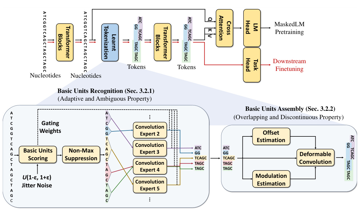
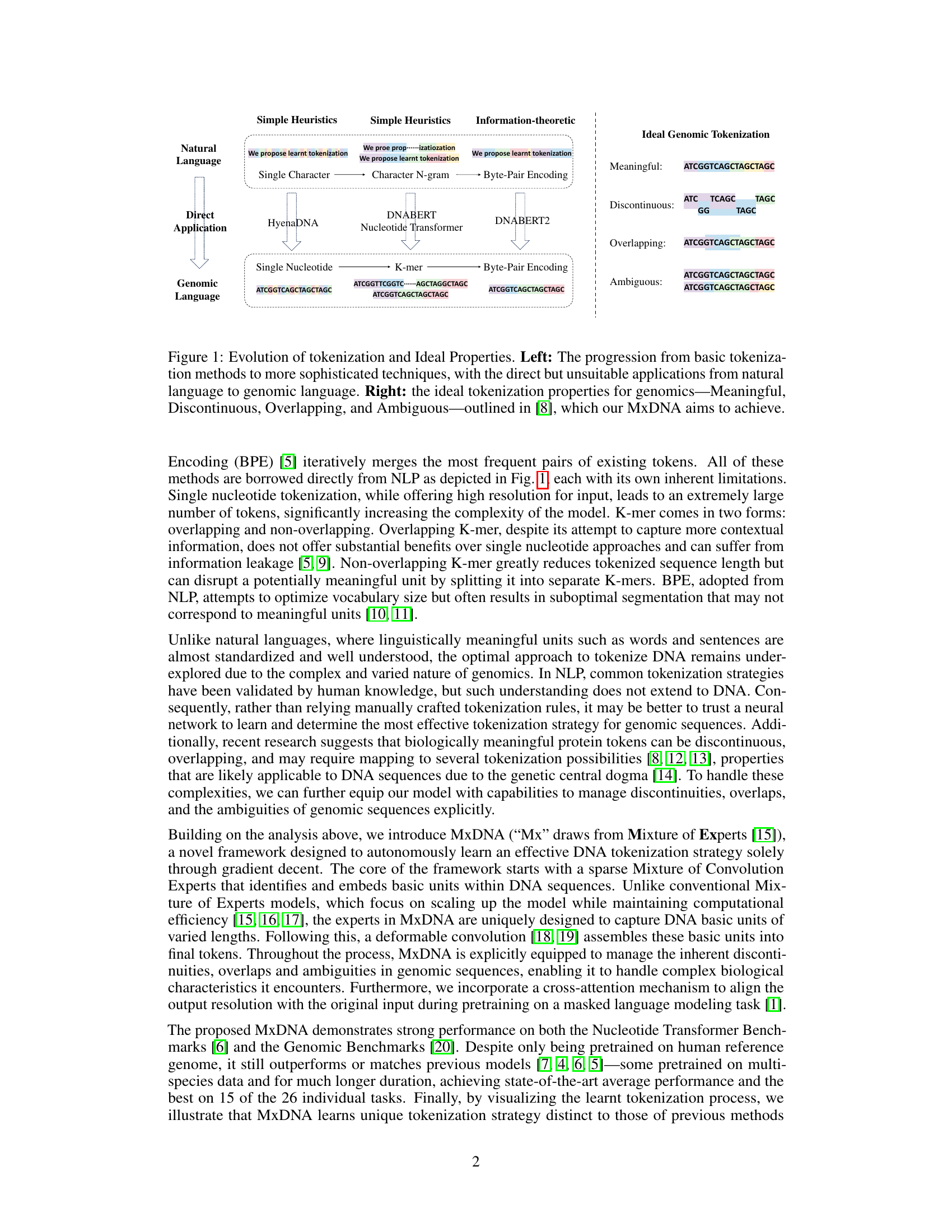
🔼 This figure illustrates the MxDNA model’s architecture and workflow. The top panel shows the overall pipeline, including pretraining and finetuning stages. The bottom panel zooms into the learned tokenization module, detailing how it identifies meaningful basic units and assembles them into final tokens using a combination of convolution experts and a deformable convolution. The process incorporates mechanisms to handle the discontinuous, overlapping, and ambiguous nature of genomic sequences.
read the caption
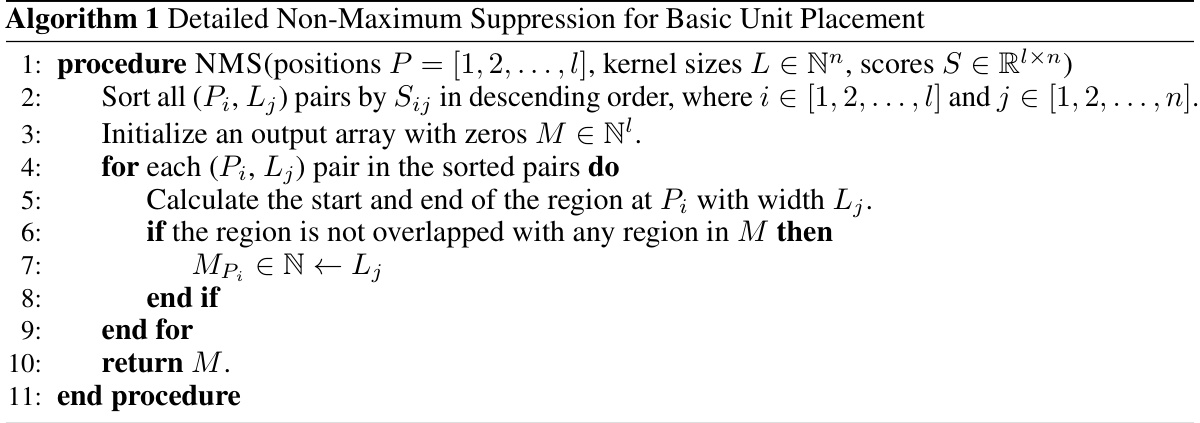
Figure 2: Our proposed MxDNA. (Top) Overall pipeline of the MxDNA model: Black arrows indicate pretraining data flow, and red arrows indicate finetuning data flow. The learnt tokenization module tokenizes single nucleotide input into learnt tokens. (Bottom) Illustration of the learnt tokenization module: Meaningful basic units are recognized with a linearly scoring layer and non-maximum suppression, embedded through convolution experts (Sec. 3.2.1), and assembled into final tokens by a deformable convolution. (Sec. 3.2.2) This process ensures meaningful, discontinuous, overlapping, and ambiguous tokenization, addressing the unique properties of genomic data.
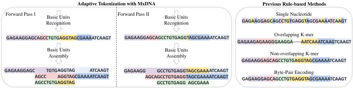
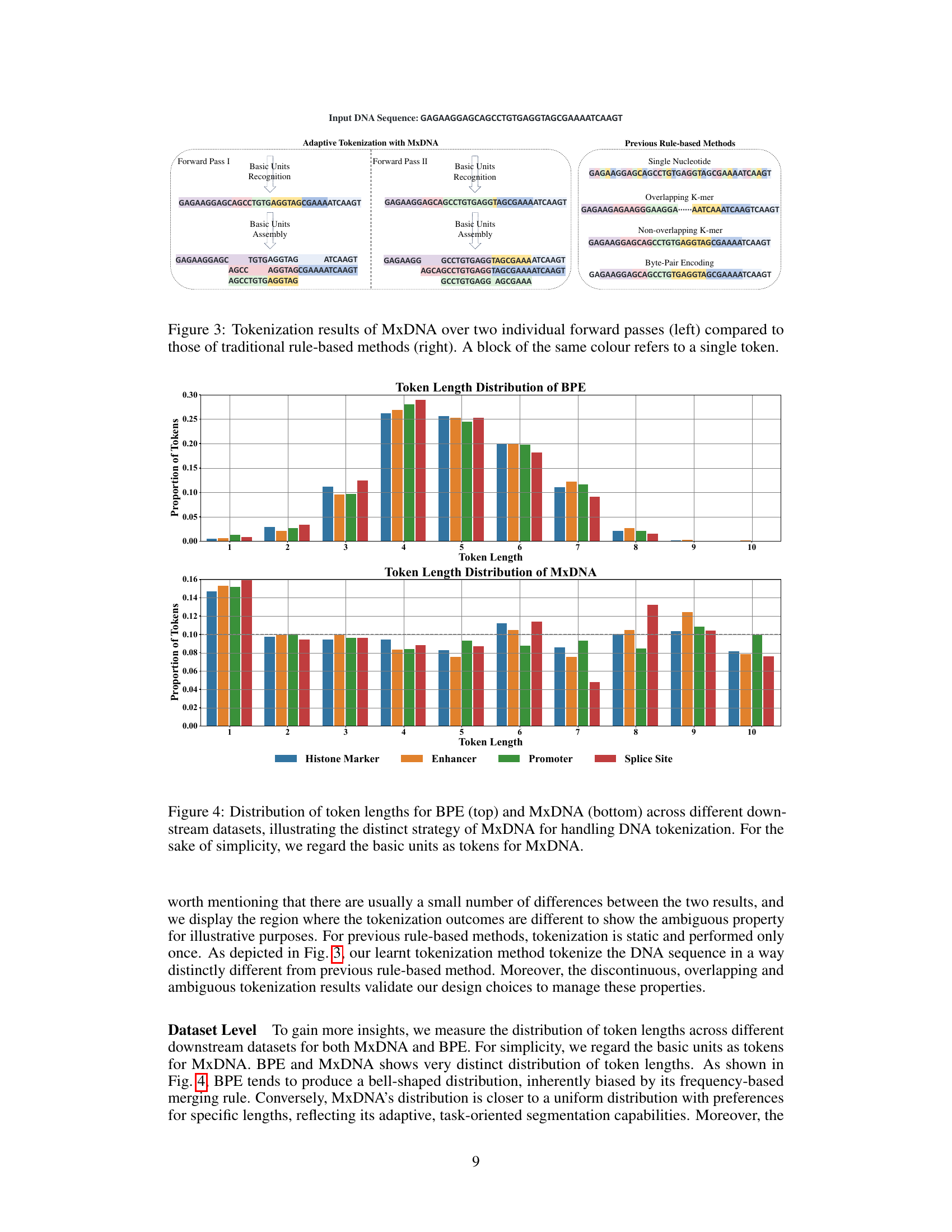
🔼 This figure compares the tokenization results of MxDNA with those of traditional methods (single nucleotide, overlapping k-mer, non-overlapping k-mer, and byte-pair encoding). MxDNA’s adaptive approach, shown in two forward passes, demonstrates its ability to identify and assemble meaningful units that may be discontinuous, overlapping, and ambiguous. In contrast, the rule-based methods show more rigid and potentially less biologically meaningful segmentations. Each coloured block represents a single token generated by each method.
read the caption
Figure 3: Tokenization results of MxDNA over two individual forward passes (left) compared to those of traditional rule-based methods (right). A block of the same colour refers to a single token.
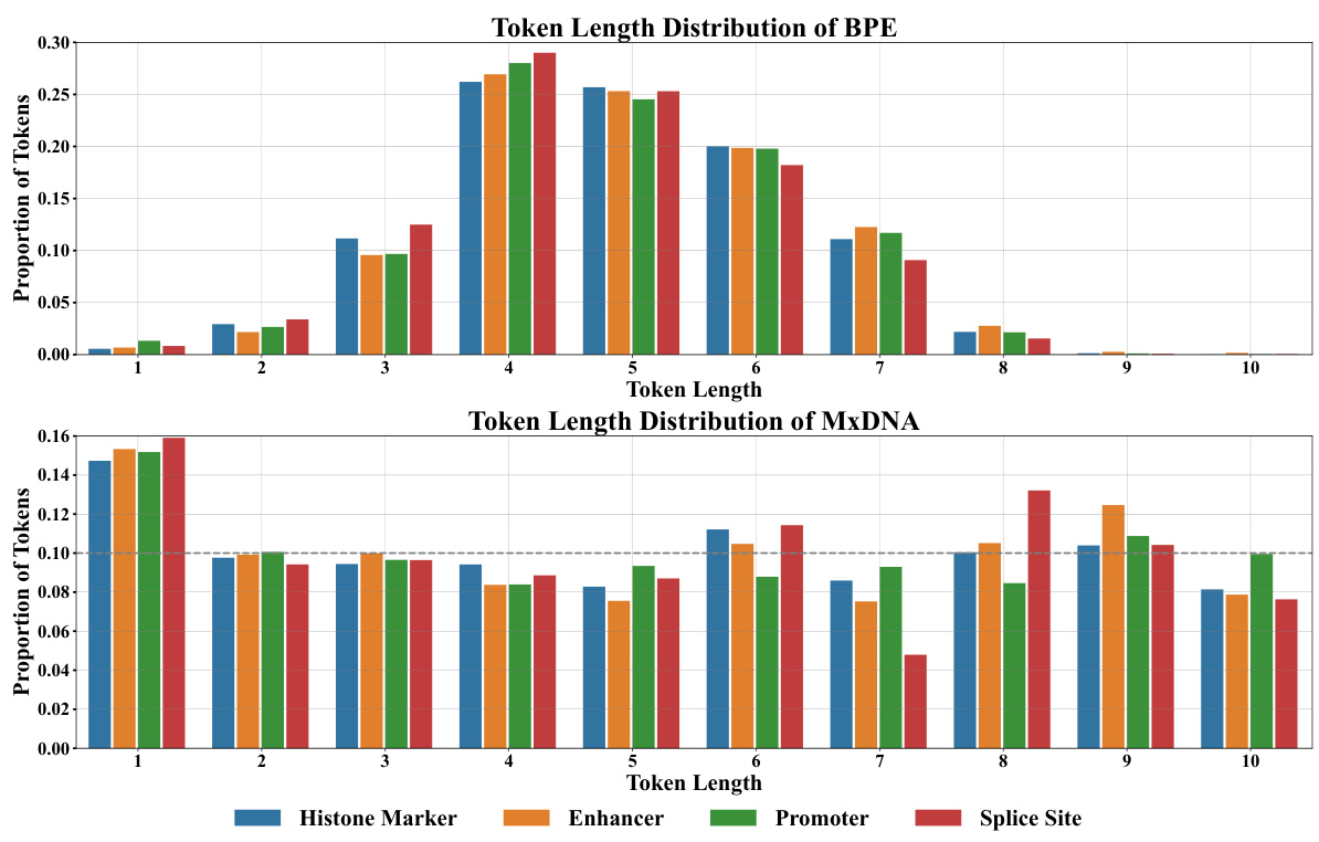
🔼 This figure compares the token length distributions of two different DNA tokenization methods: Byte-Pair Encoding (BPE) and MxDNA. The top panel shows the distribution of token lengths using BPE across four different genomic datasets (Histone Marker, Enhancer, Promoter, Splice Site). The bottom panel shows the same distribution but using the MxDNA method. The figure highlights the different strategies employed by each method, showing BPE tends to produce a bell-shaped distribution while MxDNA’s distribution is more uniform, indicating that MxDNA is more adaptive to the specific characteristics of the datasets.
read the caption
Figure 4: Distribution of token lengths for BPE (top) and MxDNA (bottom) across different downstream datasets, illustrating the distinct strategy of MxDNA for handling DNA tokenization. For the sake of simplicity, we regard the basic units as tokens for MxDNA.
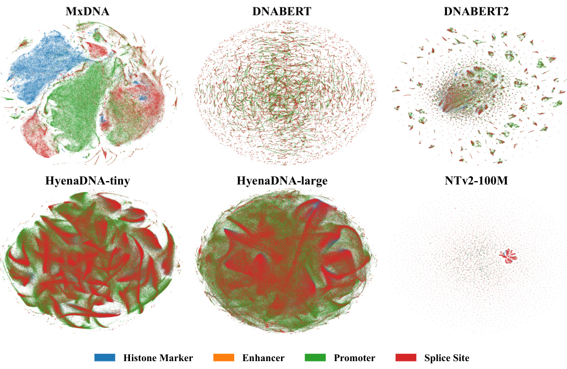
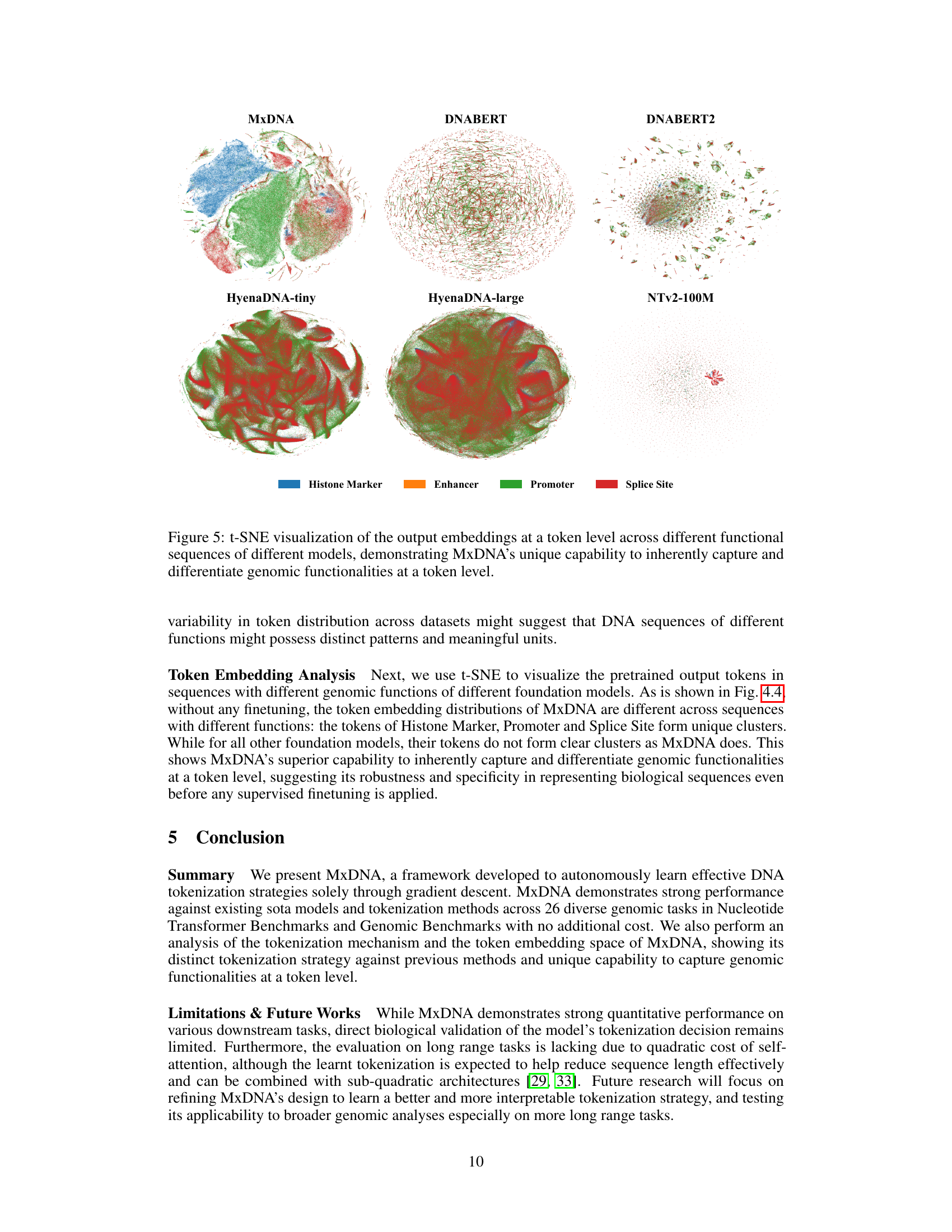
🔼 This figure shows the t-SNE visualization of the output embeddings at the token level for different foundation models including MxDNA, DNABERT, DNABERT2, HyenaDNA-tiny, HyenaDNA-large, and Nucleotide Transformer v2 100M. Each model’s embeddings are visualized separately for four different functional sequences: Histone Marker, Enhancer, Promoter, and Splice Site. The visualization aims to demonstrate MxDNA’s unique capability to inherently capture and differentiate genomic functionalities at a token level, even before any supervised finetuning is applied. The distinct clustering of different functional sequences within MxDNA’s token embedding space highlights its ability to identify and represent the underlying biological features effectively.
read the caption
Figure 5: t-SNE visualization of the output embeddings at a token level across different functional sequences of different models, demonstrating MxDNA’s unique capability to inherently capture and differentiate genomic functionalities at a token level.
More on tables
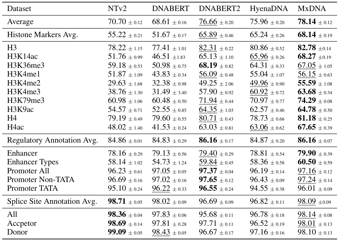
🔼 This table presents the average performance and standard deviation across three random seeds for five different DNA foundation models (Nucleotide Transformer v2 100M, DNABERT, DNABERT2, HyenaDNA, and MxDNA) on the Nucleotide Transformer Benchmarks dataset. The benchmarks encompass 18 datasets across three task types: histone marker prediction, regulatory annotation prediction, and splice site annotation prediction. The best performance for each dataset is highlighted in bold, and the second-best is underlined.
read the caption
Table 2: Nucleotide Transformer Benchmarks. Average performance across three random seeds for Nucleotide Transformer v2 100M, DNABERT, DNABERT2, HyenaDNA and MxDNA with sample standard deviations. We highlight the best values in bold type and underline the second best.
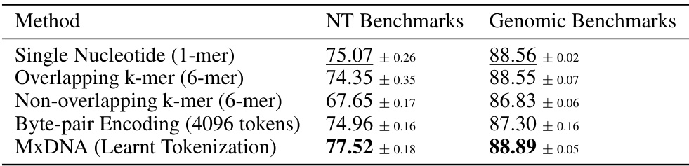
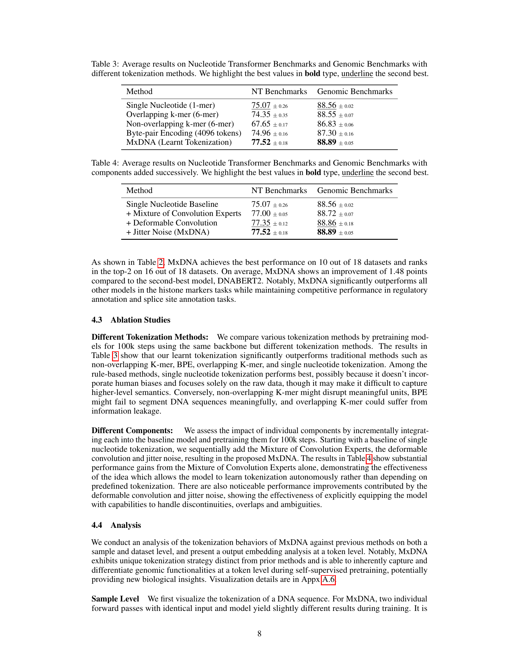
🔼 This table compares the performance of different DNA tokenization methods on two benchmark datasets: Nucleotide Transformer Benchmarks and Genomic Benchmarks. The methods compared include Single Nucleotide, Overlapping k-mer, Non-overlapping k-mer, Byte-pair Encoding, and the proposed MxDNA method. The table shows that MxDNA outperforms other methods on both benchmarks. The average performance and standard deviations are presented for each method.
read the caption
Table 3: Average results on Nucleotide Transformer Benchmarks and Genomic Benchmarks with different tokenization methods. We highlight the best values in bold type, underline the second best.
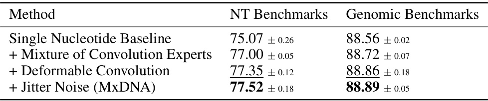
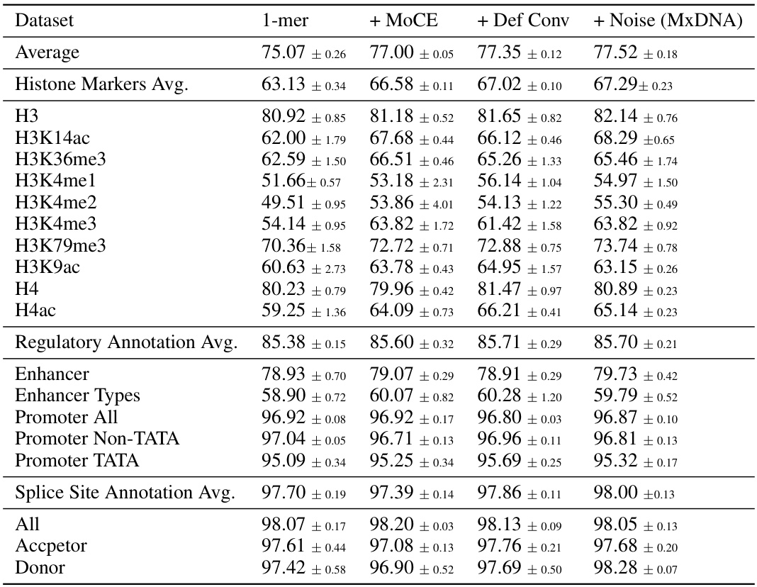
🔼 This table shows the impact of adding different components to the MxDNA model. It starts with a baseline of single nucleotide tokenization and then adds the Mixture of Convolution Experts, the deformable convolution and jitter noise sequentially. Each row shows the average performance on both Nucleotide Transformer and Genomic Benchmarks after each component addition. The results demonstrate that each component contributes to improved performance, culminating in the final MxDNA model.
read the caption
Table 4: Average results on Nucleotide Transformer Benchmarks and Genomic Benchmarks with components added successively. We highlight the best values in bold type, underline the second best.
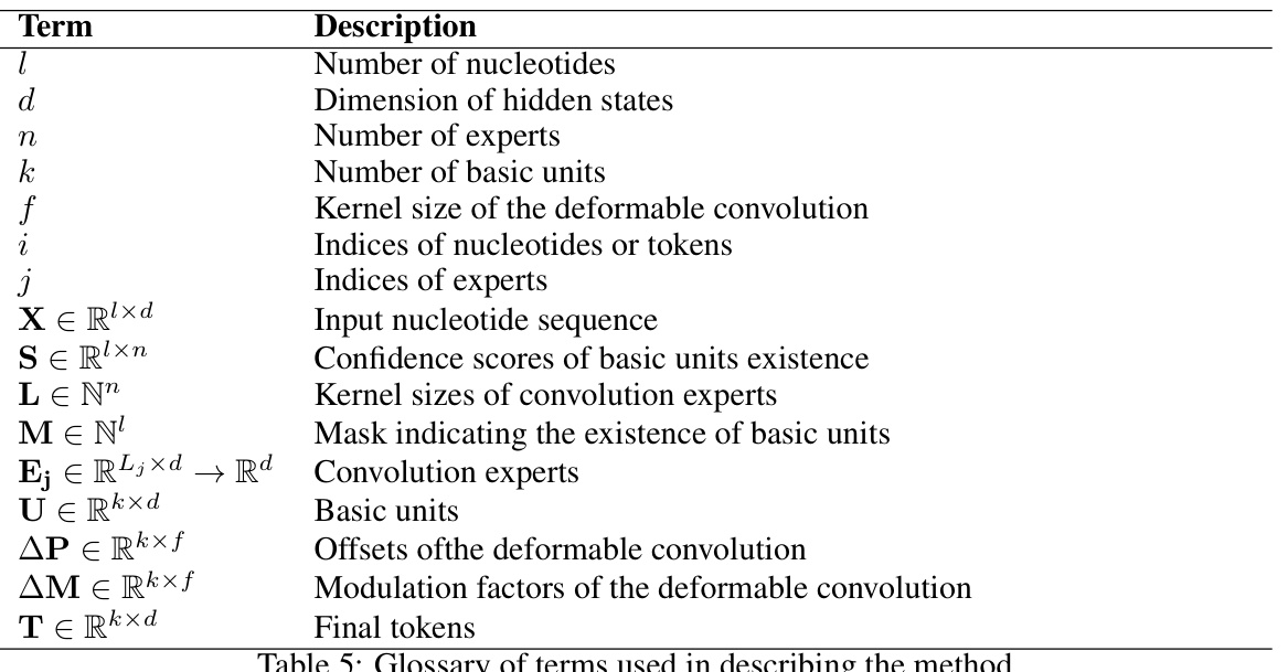
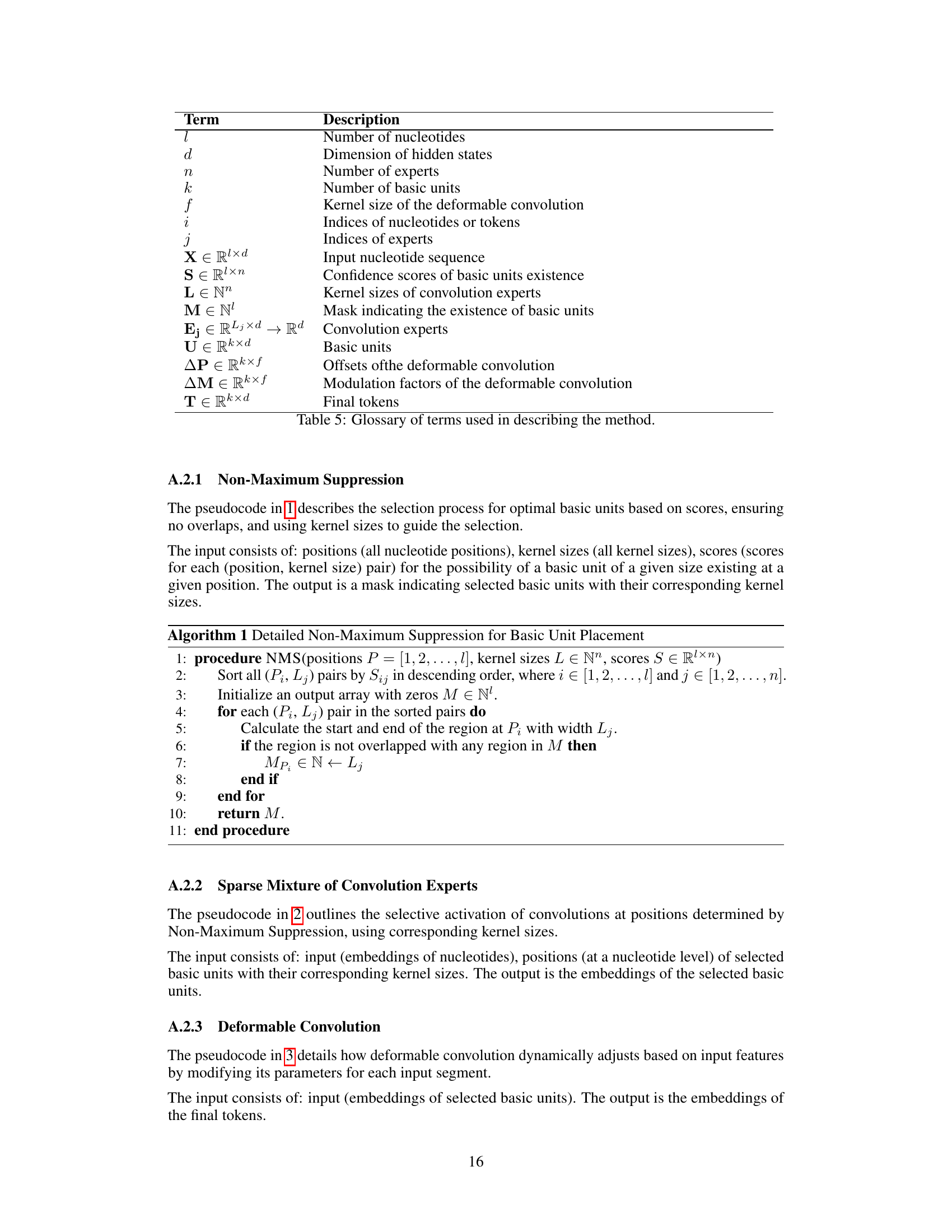
🔼 This table provides a glossary of terms and their descriptions used in the paper’s methodology section. It defines key variables such as the number of nucleotides, dimension of hidden states, number of experts, etc., along with their data types and meanings within the context of MxDNA.
read the caption
Table 5: Glossary of terms used in describing the method.
🔼 This table compares the average performance of five different DNA foundation models (Nucleotide Transformer v2 100M, DNABERT, DNABERT2, HyenaDNA, and MxDNA) across eight genomic benchmark datasets. The best performing model for each dataset is highlighted in bold, and the second-best is underlined. The results show MxDNA’s superior performance on several benchmarks.
read the caption
Table 1: Genomic Benchmarks. Average performance across three random seeds for Nucleotide Transformer v2 100M, DNABERT, DNABERT2, HyenaDNA and MxDNA with sample standard deviations. We highlight the best values in bold type and underline the second best.
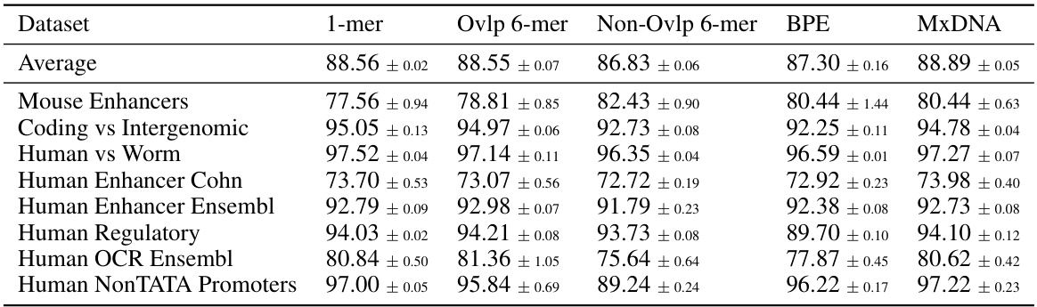
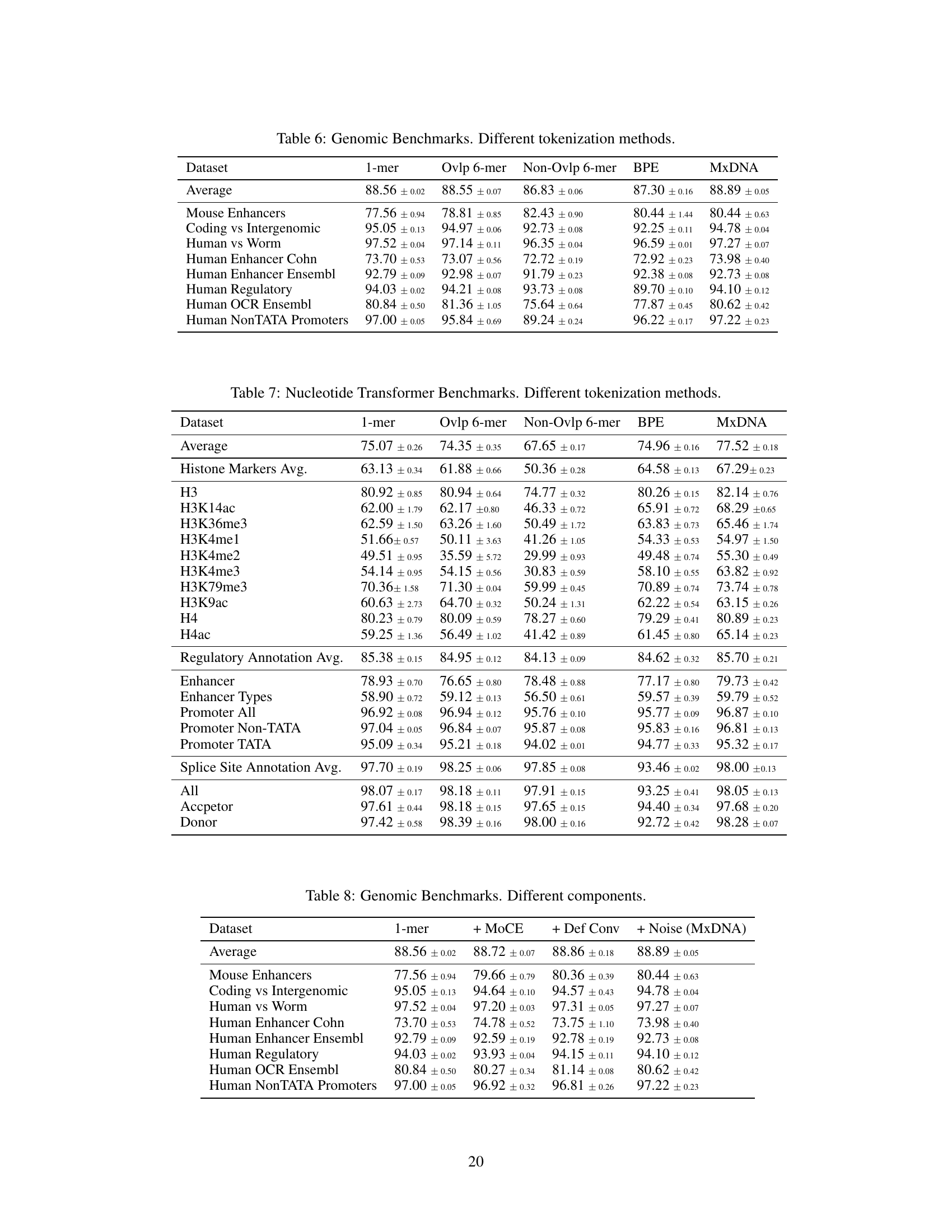
🔼 This table compares the performance of different DNA tokenization methods (single nucleotide, overlapping 6-mer, non-overlapping 6-mer, Byte Pair Encoding, and MxDNA) on eight genomic tasks. The performance metric used is average accuracy across three random seeds. The table showcases how MxDNA outperforms other methods in most tasks.
read the caption
Table 6: Genomic Benchmarks. Different tokenization methods.
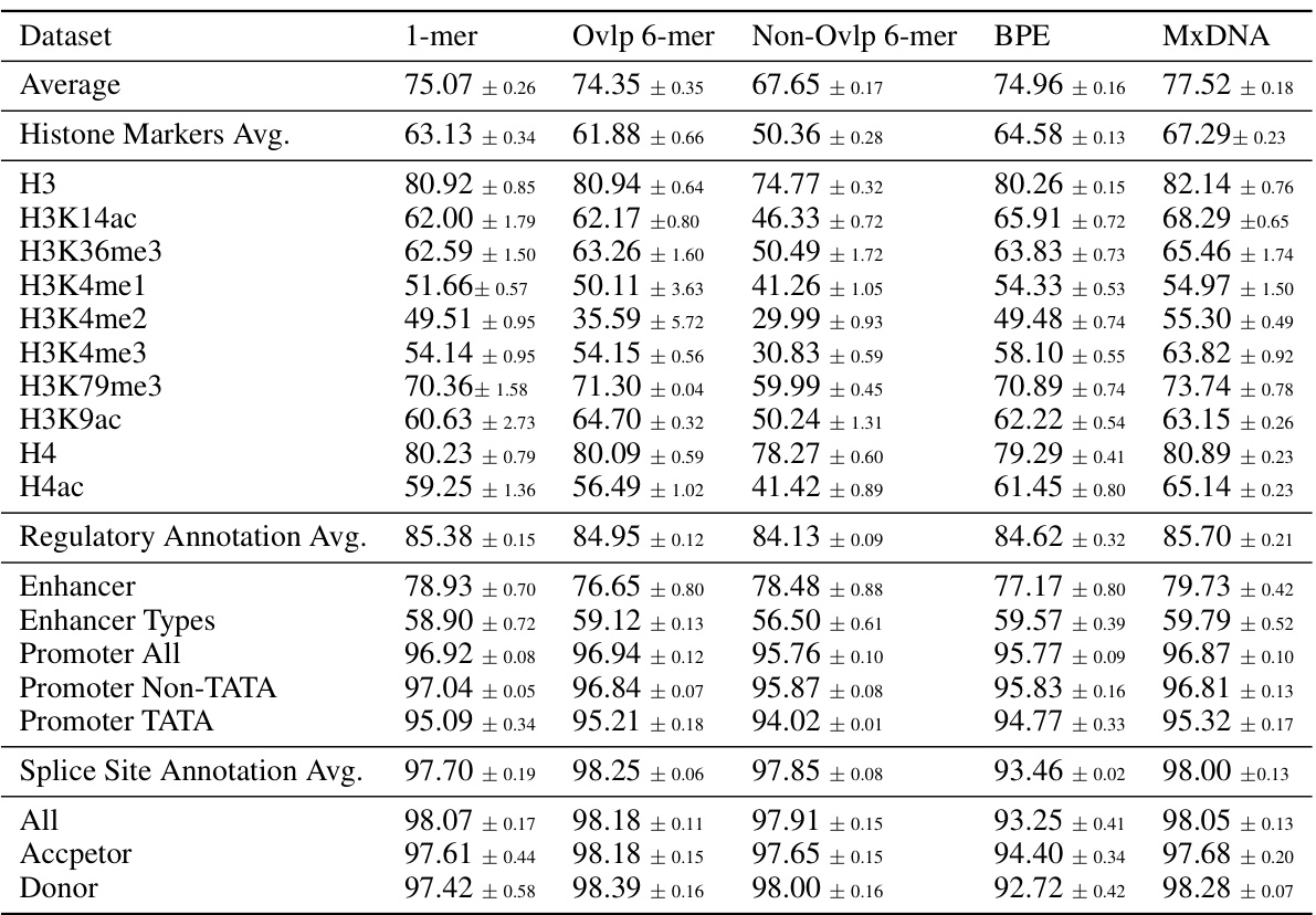
🔼 This table presents the average performance across three random seeds for different DNA tokenization methods on the Nucleotide Transformer Benchmarks. The methods compared include single nucleotide (1-mer), overlapping 6-mer, non-overlapping 6-mer, Byte-Pair Encoding (BPE), and the proposed MxDNA method. The results are shown for various downstream tasks, including histone marker prediction, regulatory annotation, and splice site annotation, demonstrating the performance of MxDNA against other tokenization approaches.
read the caption
Table 7: Nucleotide Transformer Benchmarks. Different tokenization methods.
🔼 This table presents the average performance results on Genomic Benchmarks for different model configurations. It compares the performance of a single nucleotide baseline model against models with progressively added components: Mixture of Convolution Experts, Deformable Convolution, and finally, Jitter Noise (resulting in the full MxDNA model). The results show how each component contributes to the overall improved performance.
read the caption
Table 8: Genomic Benchmarks. Different components.
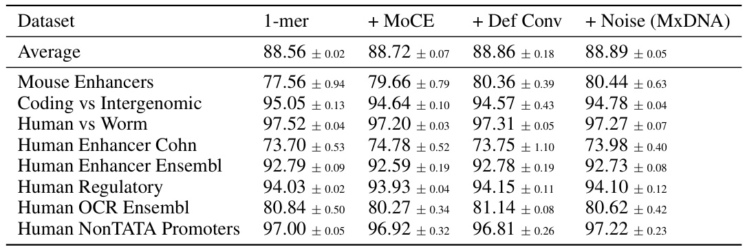
🔼 This table presents the average results on Nucleotide Transformer Benchmarks with components added successively to the single nucleotide baseline. It shows the performance improvements with the addition of the Mixture of Convolution Experts, deformable convolution, and jitter noise, culminating in the final MxDNA model. Each row represents a specific dataset or average across multiple datasets within the benchmarks, and each column shows the performance with a progressively more complete version of the model.
read the caption
Table 9: Nucleotide Transformer Benchmarks. Different components.
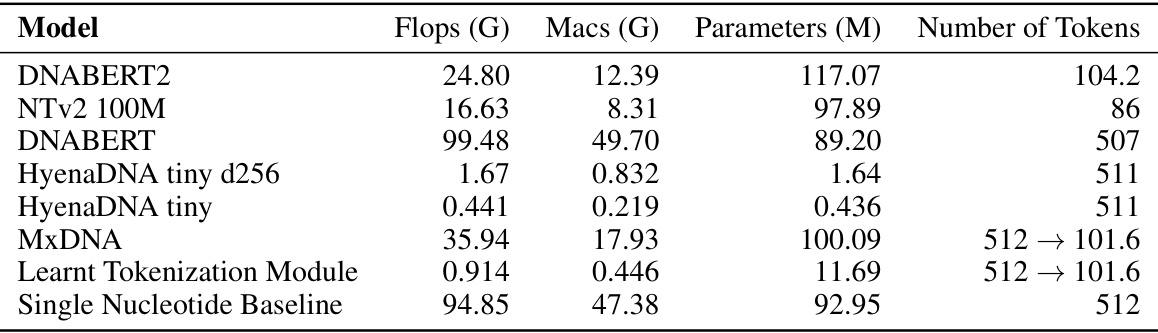
🔼 This table compares several DNA foundation models (DNABERT2, Nucleotide Transformer v2 100M, DNABERT, HyenaDNA tiny d256, HyenaDNA tiny, MxDNA, Learnt Tokenization Module, Single Nucleotide Baseline) across four key metrics reflecting their computational complexity: floating point operations (FLOPs), multiply-accumulate operations (MACs), number of parameters, and the number of tokens. The table allows for a quantitative assessment of the relative computational resource requirements of each model.
read the caption
Table 10: Comparison of various models based on their computational complexity.
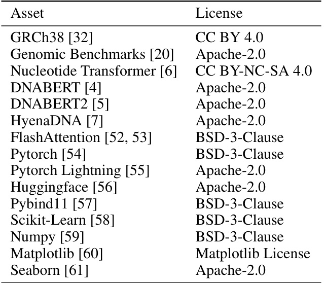
🔼 This table lists the various assets (datasets, models, libraries, etc.) used in the research, along with their respective licenses. It provides transparency regarding the source and usage rights of the components that contribute to the overall methodology and results.
read the caption
Table 11: Assets used in this work
Full paper#