TL;DR#
Persistent homology is a powerful tool for analyzing the shape of data, but it often fails when dealing with high-dimensional data containing noise. This is because in high dimensions, the distances between data points become less informative, making it difficult to identify meaningful topological structures. Existing solutions haven’t effectively addressed this “curse of dimensionality.”
This research tackles this problem by using spectral distances on a k-nearest neighbor graph of the data. Spectral distances, such as effective resistance and diffusion distance, are more robust to noise in high dimensions because they consider the overall structure of the data, rather than just individual point-to-point distances. The researchers demonstrate that this approach significantly improves the accuracy of persistent homology in high-dimensional noisy datasets, particularly in the context of analyzing single-cell RNA sequencing data where it successfully detects cell cycle loops.
Key Takeaways#
Why does it matter?#
This paper is crucial for researchers working with high-dimensional data because it introduces a novel approach to persistent homology that overcomes the limitations of traditional methods in handling high-dimensional noise. This is highly relevant to many fields dealing with such data and opens up new avenues for topological analysis.
Visual Insights#

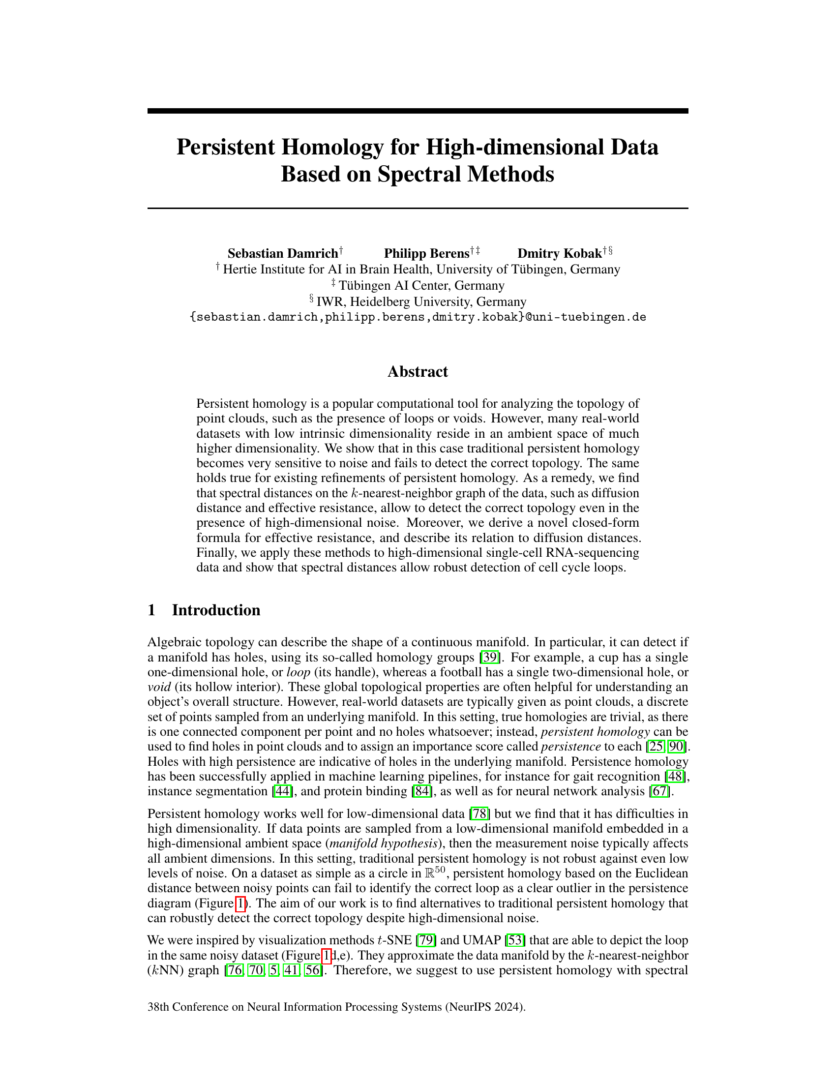
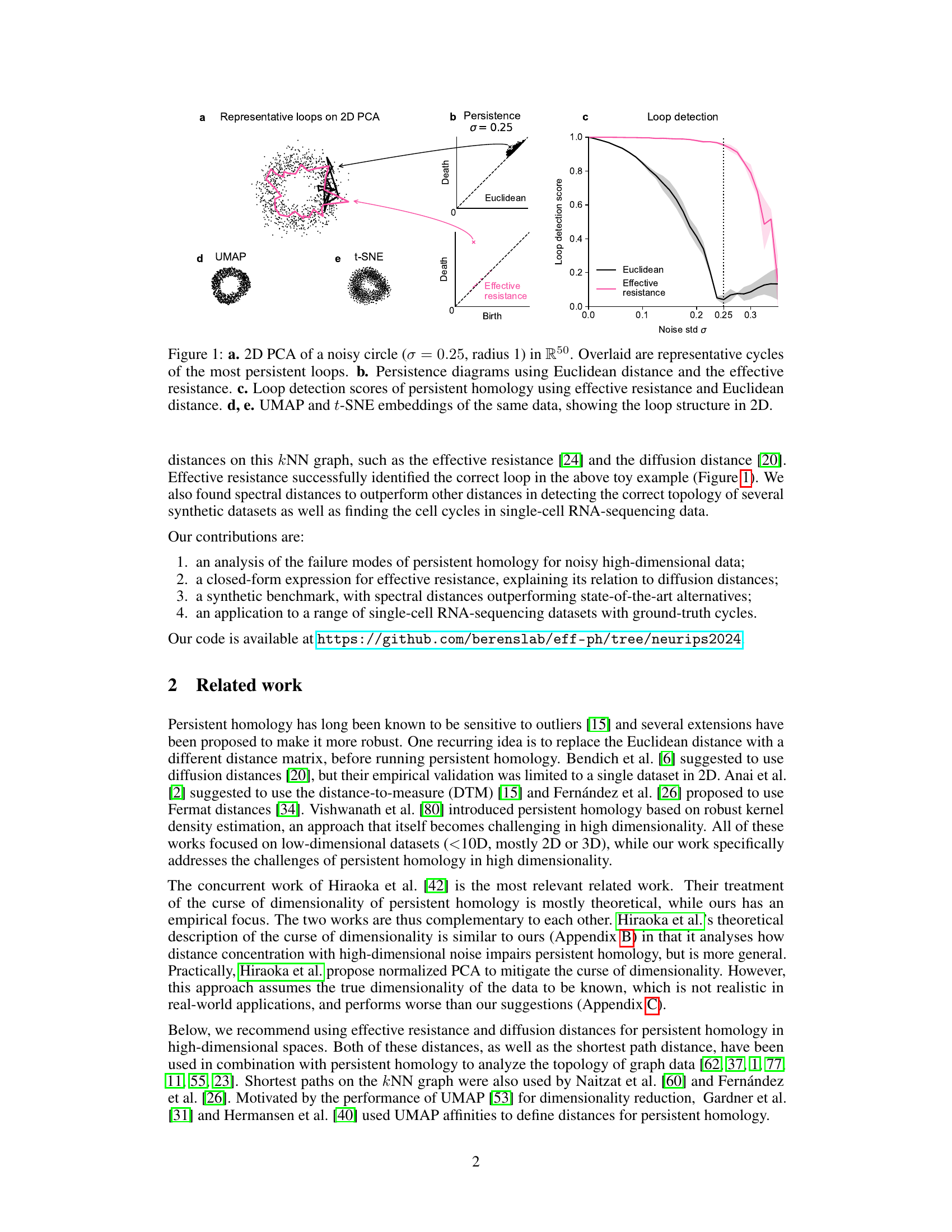
🔼 This figure compares different methods for detecting topological features (loops) in noisy high-dimensional data. Panel (a) shows a 2D PCA projection of a noisy circle embedded in 50 dimensions, with representative loops identified by persistent homology using Euclidean distance. Panel (b) presents persistence diagrams illustrating the performance of both Euclidean distance and effective resistance in identifying the loop structure. Panel (c) quantitatively assesses the loop detection scores for both methods across various noise levels (σ). Finally, panels (d) and (e) display the same data using UMAP and t-SNE dimensionality reduction techniques, respectively, demonstrating that low-dimensional embeddings reveal the loop structure, even when Euclidean distance-based persistent homology fails.
read the caption
Figure 1: a. 2D PCA of a noisy circle (σ = 0.25, radius 1) in R50. Overlaid are representative cycles of the most persistent loops. b. Persistence diagrams using Euclidean distance and the effective resistance. c. Loop detection scores of persistent homology using effective resistance and Euclidean distance. d, e. UMAP and t-SNE embeddings of the same data, showing the loop structure in 2D.

🔼 This table presents the best hyperparameter settings for different distance measures used in persistent homology analysis, as determined by their performance in Figure 7 of the paper. The hyperparameters are specific to different datasets (Circle, Eyeglasses, Linked Circles, Torus, Sphere) and topological feature types (loops, voids). The table shows the optimal settings for Fermat distance (parameter ‘p’), DTM distance (parameters ‘k’, ‘p’, ‘ξ’), effective resistance distance (parameter ‘k’), and diffusion distance (parameters ‘k’, ’t’). These optimal settings were chosen based on maximizing the performance of persistent homology for detecting topological features, allowing for better understanding and reproducibility of the results in the paper.
read the caption
Table S1: The optimal hyperparameters that were selected in Figure 7. For torus and sphere, we consider the case of loop detection (H1) and void detection (H2) separately.
In-depth insights#
High-D Homology#
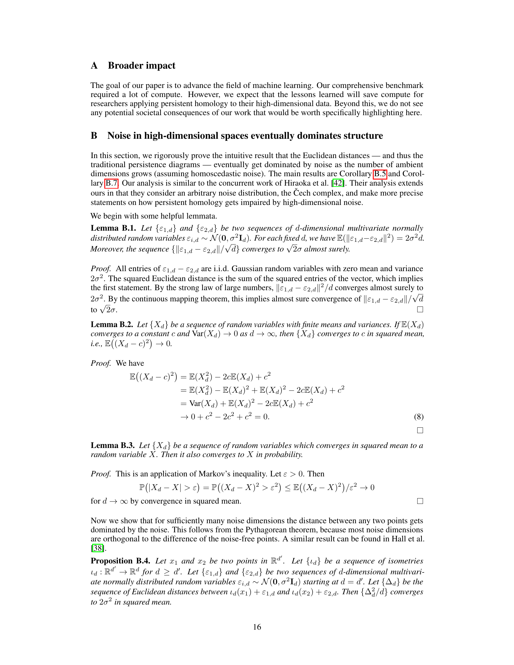
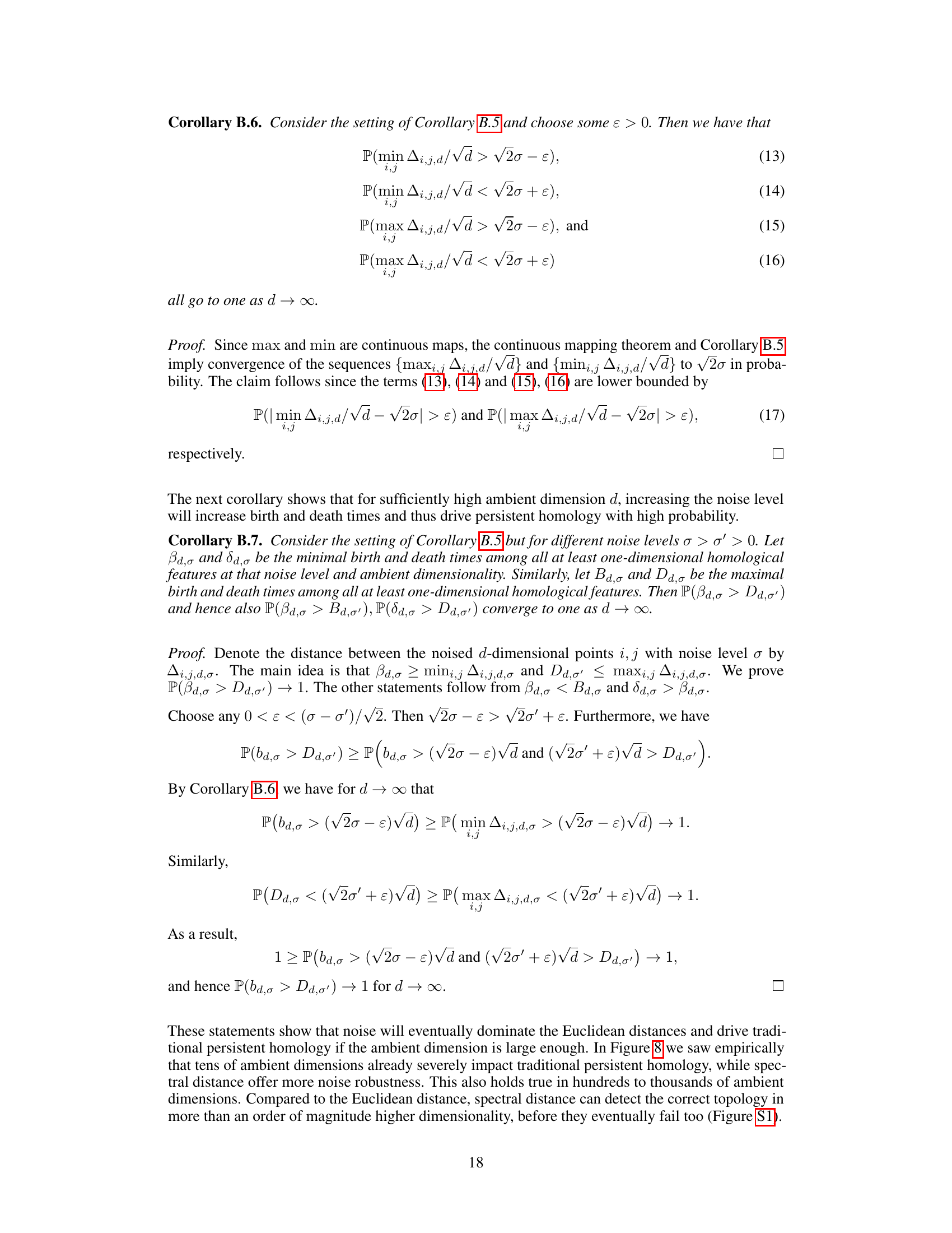
The concept of “High-D Homology” refers to the application of persistent homology to high-dimensional datasets. Traditional persistent homology struggles in high dimensions due to the curse of dimensionality, where noise overwhelms the underlying topological structure. The paper addresses this challenge by proposing the use of spectral distances (such as diffusion distance and effective resistance) calculated on k-nearest neighbor graphs. These spectral methods are shown to be more robust to high-dimensional noise and better at identifying true topological features. The authors demonstrate that these approaches outperform conventional methods in both synthetic and real-world single-cell RNA sequencing datasets. Closed-form expressions for spectral distances, and a novel relationship to diffusion distances, enhance understanding and computational efficiency. The key is that the local structure captured by kNN graphs is preserved even when global distances are obscured by high dimensionality. The paper’s work has implications for fields dealing with high-dimensional data where understanding the underlying shape is critical for interpretation.
Spectral Distances#
The concept of spectral distances within the context of high-dimensional data analysis and persistent homology is crucial. Traditional methods struggle with noise in high dimensions, but spectral distances, such as diffusion distance and effective resistance, leverage the structure of the k-nearest-neighbor graph. This graph-based approach is robust to high-dimensional noise because it focuses on local relationships, which are less affected by noise than global distances. The authors derive a novel closed-form expression for effective resistance, linking it directly to diffusion distances. This is significant because it provides a clear theoretical understanding of how spectral distances relate to each other and highlights their importance in persistent homology. The empirical results show that persistent homology using spectral distances consistently outperforms traditional methods when dealing with high-dimensional noisy datasets, making spectral distances a vital tool for topological data analysis in challenging settings.
Cell Cycle Loops#
The concept of “Cell Cycle Loops” in the context of single-cell RNA sequencing (scRNA-seq) data analysis, using persistent homology, is intriguing. The cell cycle is not a linear process; it’s cyclical, with cells progressing through various phases (G1, S, G2, M) before dividing. Persistent homology, a topological data analysis technique, can effectively capture this cyclical nature by identifying loops or cycles within the high-dimensional scRNA-seq data. These loops represent groups of cells exhibiting similar gene expression patterns characteristic of particular cell cycle phases. The presence and strength of these loops can then provide insights into cell cycle dynamics, potentially revealing variations in cell cycle progression among different cell populations or under varying conditions. The challenge lies in the high dimensionality and noise inherent in scRNA-seq data. The authors address this with spectral methods, such as diffusion distance and effective resistance, to construct more robust representations of cell-cell relationships before applying persistent homology. This approach enhances the detection and interpretation of cell cycle loops, offering a powerful means to study cell cycle regulation and its relation to cellular processes. Robustness to noise is a significant advantage of the spectral method used, ensuring reliable results even with biological variation.
Limitations#
The limitations section of this research paper should thoughtfully address several key aspects. Firstly, it must acknowledge the inherent challenges in automatically evaluating the correctness of identified topological cycles, particularly in real-world datasets with complex structures. Secondly, it should explicitly state the reliance on the k-nearest-neighbor graph, emphasizing potential biases introduced by parameter choices (k-value selection). Thirdly, the computational cost associated with persistent homology, especially for high-dimensional data and large sample sizes, should be clearly highlighted along with the scaling limitations. Finally, it is crucial to discuss the limitations of relying solely on topological information, as it might not fully capture important non-topological features or differentiate between non-isomorphic point clouds with similar topology. A robust limitations section would enhance the paper’s overall credibility by acknowledging these factors and offering perspectives on future improvements.
Future Work#
The authors suggest several avenues for future research. Extending the theoretical analysis to formally prove that spectral distances mitigate the curse of dimensionality is crucial. Investigating the stability of spectral distances under different noise models and data distributions would provide further robustness. The authors also suggest the exploration of spectral methods beyond high-dimensional single-cell RNA-sequencing data, in areas such as artificial neural networks, climate science, and astronomy. Improving the efficiency of persistent homology computation with spectral distances, perhaps through subsampling techniques, remains a significant challenge. Finally, developing automated methods for evaluating the correctness of detected cycles in real-world applications, which is currently limited by manual inspection, is a key area for future work.
More visual insights#
More on figures

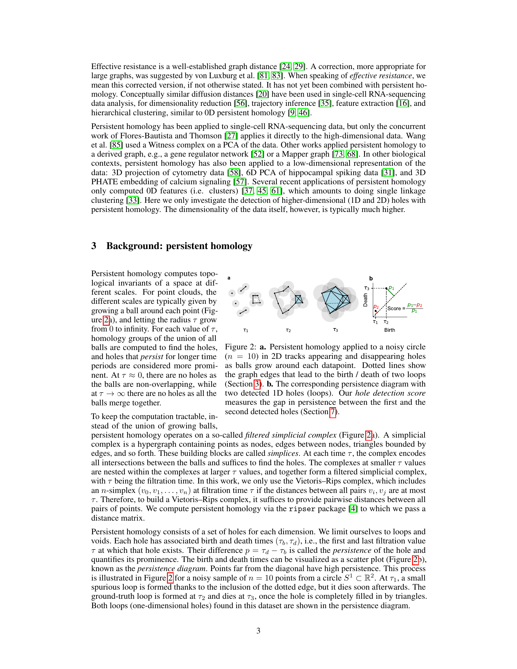
🔼 This figure illustrates the concept of persistent homology using a simple example of a noisy circle with 10 points in a 2D space. Part (a) shows how the algorithm tracks the appearance and disappearance of holes as it grows balls around data points, with dotted lines representing graph edges that lead to the creation or destruction of loops. Part (b) displays the resulting persistence diagram showing the two detected 1D holes (loops) and their persistence values. The hole detection score is then introduced to quantify the prominence of these holes by measuring the gap between persistence values.
read the caption
Figure 2: a. Persistent homology applied to a noisy circle (n = 10) in 2D tracks appearing and disappearing holes as balls grow around each datapoint. Dotted lines show the graph edges that lead to the birth / death of two loops (Section 3). b. The corresponding persistence diagram with two detected 1D holes (loops). Our hole detection score measures the gap in persistence between the first and the second detected holes (Section 7).

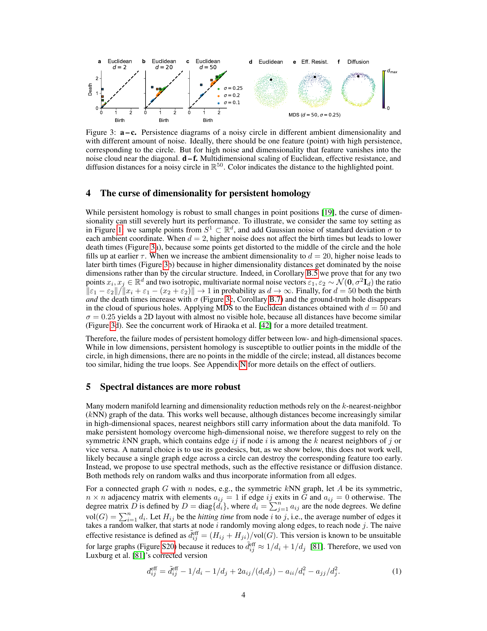
🔼 This figure demonstrates how persistent homology using Euclidean distance fails in high-dimensional noisy data. Panels (a-c) show persistence diagrams of a noisy circle embedded in spaces of increasing dimensionality (d=2, 20, 50). As noise and dimensionality increase, the feature representing the circle becomes less distinct and eventually indistinguishable from the noise. Panels (d-f) show multidimensional scaling (MDS) plots of the same noisy circle in 50 dimensions (σ = 0.25) using three different distances: Euclidean, effective resistance, and diffusion distance. The color-coding highlights how effective resistance and diffusion distances are more robust to high-dimensional noise, preserving the loop structure of the circle more effectively than Euclidean distance.
read the caption
Figure 3: a-c. Persistence diagrams of a noisy circle in different ambient dimensionality and with different amount of noise. Ideally, there should be one feature (point) with high persistence, corresponding to the circle. But for high noise and dimensionality that feature vanishes into the noise cloud near the diagonal. d-f. Multidimensional scaling of Euclidean, effective resistance, and diffusion distances for a noisy circle in R50. Color indicates the distance to the highlighted point.

🔼 This figure compares the robustness of geodesic distance and effective resistance to random edges added to a k-NN graph constructed from points sampled from a noisy circle. The geodesic distance, which follows the shortest path, is highly susceptible to these added edges, drastically altering the distance calculations. Conversely, the effective resistance distance remains largely unaffected, highlighting its robustness.
read the caption
Figure 4: Robustness of effective resistance. We sampled n = 1000 points from a noisy circle in 2D with Gaussian noise of standard deviation σ = 0.1, constructed the unweighted symmetric 15-NN graph, and optionally added 10 random edges (thick lines). Node colors indicate the graph distance from the fat black dot. a. The geodesic distance is severely affected by the random edges. b. The effective resistance distance is robust to them.

🔼 Figure 5 shows the eigenvalue spectra of the kNN graph Laplacian for a noisy circle in 50-dimensional ambient space with different noise levels (σ = 0.0, 0.1, 0.25). It also illustrates the decay of eigenvector contribution based on the eigenvalue for several distance measures (effective resistance, diffusion distances, and diffusion pseudotime). Finally, it presents the relative contribution of each eigenvector for these distance measures at various noise levels, highlighting their differences in how they incorporate information from different scales of the graph.
read the caption
Figure 5: a. Eigenvalue spectra of the kNN graph Laplacian for the noisy circle in ambient R50 for noise levels σ = {0.0, 0.1, 0.25}. b. Decay of eigenvector contribution based on the eigenvalue for effective resistance, diffusion distances and DPT. c-e. Relative contribution of each eigenvector for eff. resistance, diffusion distance, Laplacian Eigenmaps, and DPT for various noise levels (Section 6).

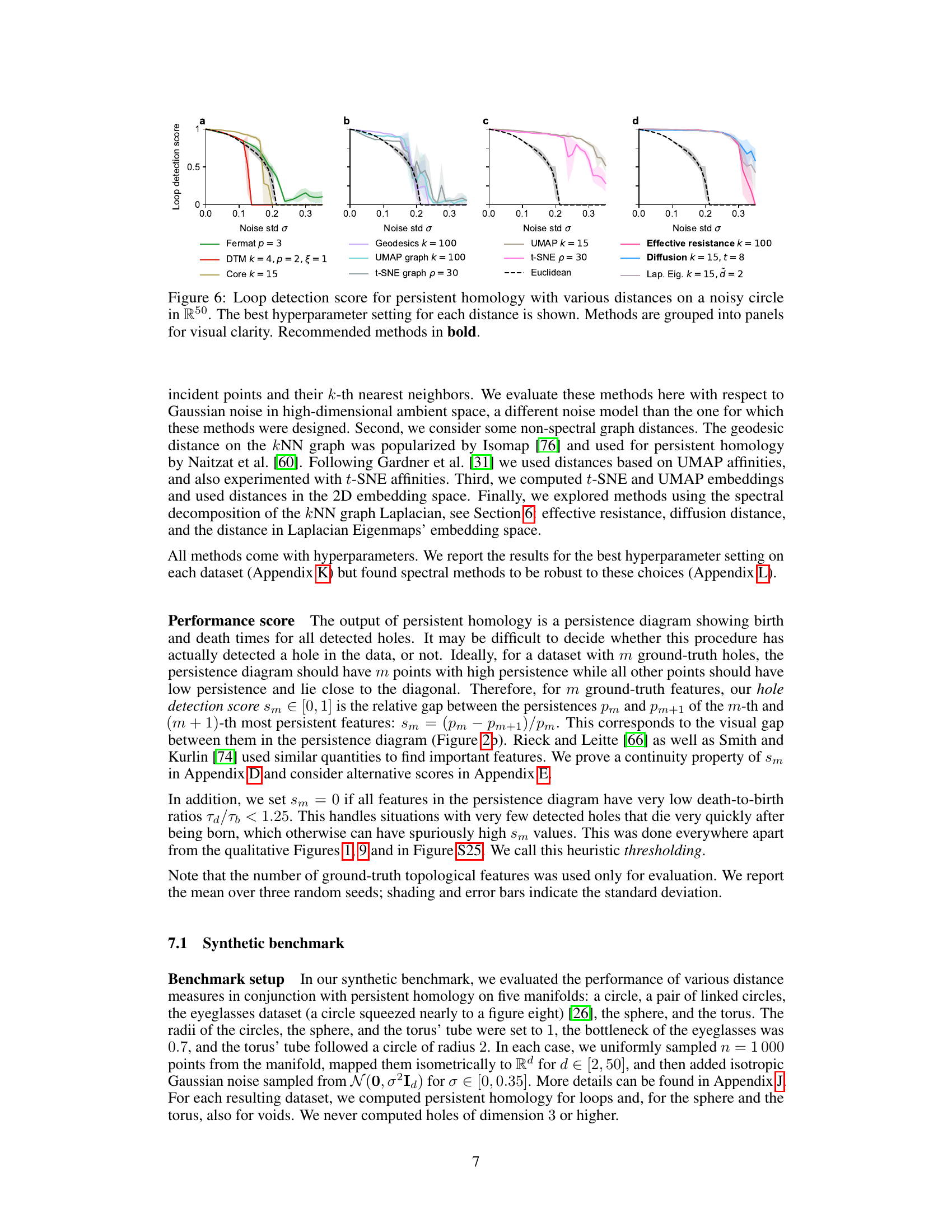
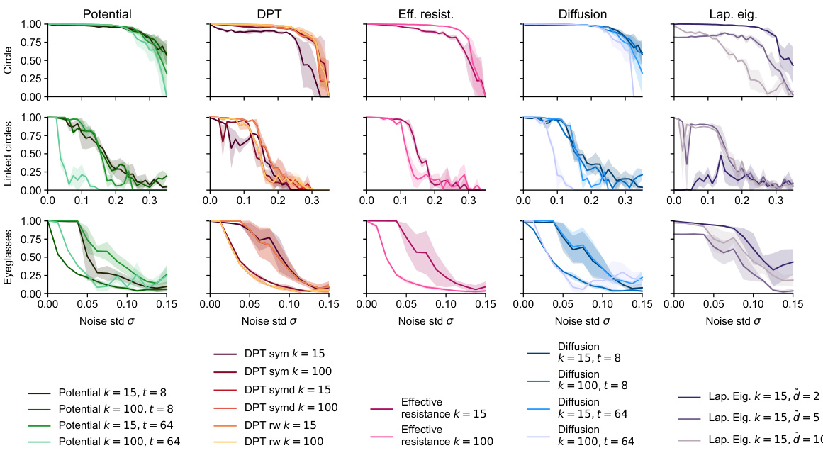
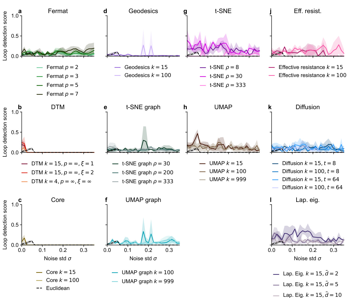
🔼 This figure compares the performance of various distance metrics used in persistent homology for detecting a loop in a noisy dataset. The x-axis shows the level of noise (standard deviation of Gaussian noise added to a circle in 50 dimensions), and the y-axis shows the loop detection score, a measure of how successfully persistent homology identified the loop. The figure highlights that spectral methods, such as effective resistance and diffusion distances, are more robust to noise than traditional Euclidean distance and other methods.
read the caption
Figure 6: Loop detection score for persistent homology with various distances on a noisy circle in R50. The best hyperparameter setting for each distance is shown. Methods are grouped into panels for visual clarity. Recommended methods in bold.
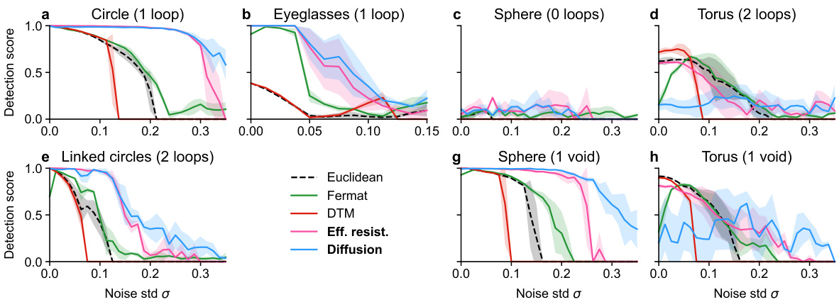
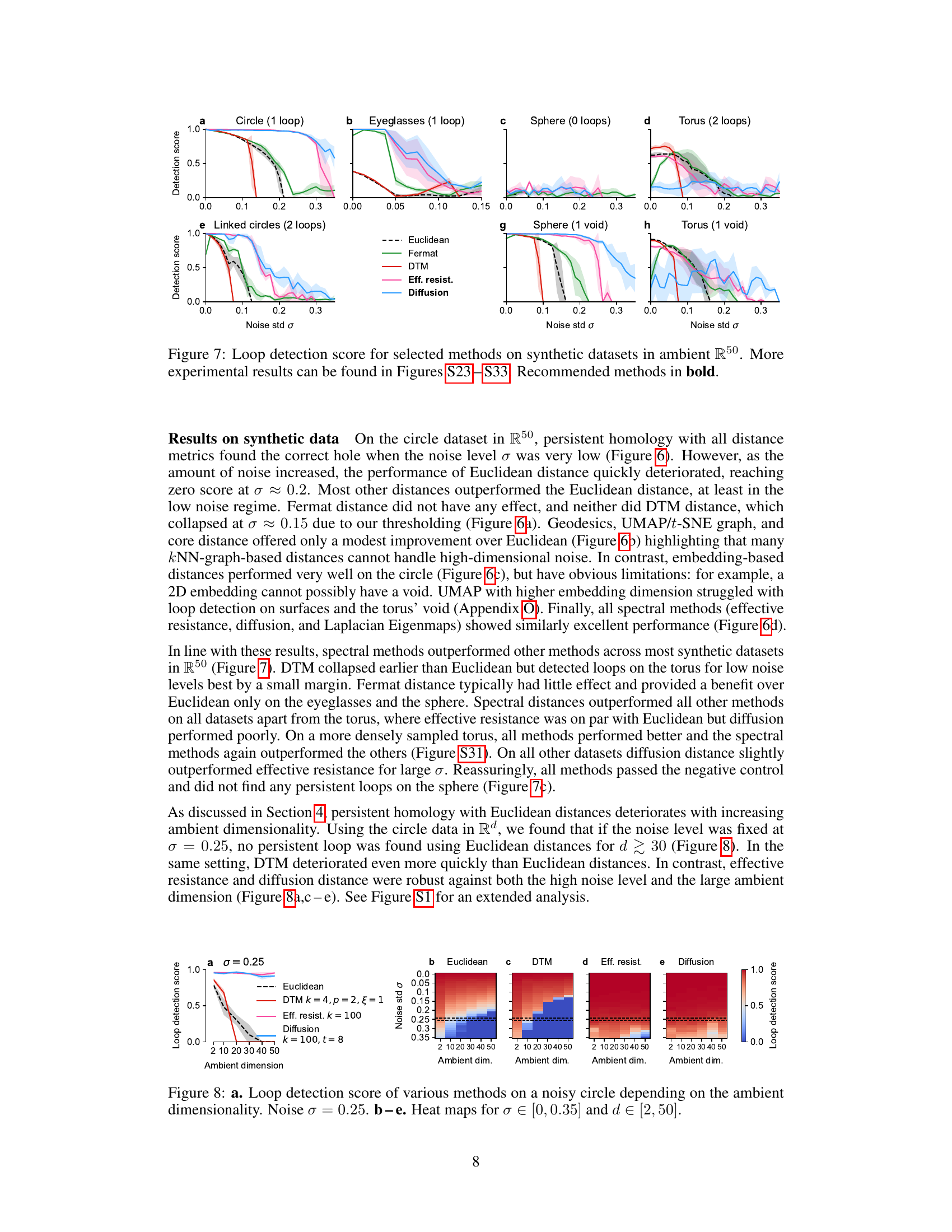
🔼 This figure compares the performance of several methods for detecting loops in synthetic datasets with varying levels of noise in a 50-dimensional ambient space. The x-axis represents the standard deviation (σ) of added Gaussian noise, and the y-axis represents the loop detection score, a metric indicating the success of the method in identifying the correct loop structure. Each line represents a different distance metric (Euclidean, Fermat, DTM, effective resistance, diffusion) used as input to persistent homology to analyze the noisy data. The figure shows that spectral distances (effective resistance and diffusion) generally outperform other methods, particularly at higher noise levels. The best-performing methods for each dataset are highlighted in bold, signifying their superior robustness to high-dimensional noise.
read the caption
Figure 7: Loop detection score for selected methods on synthetic datasets in ambient R50. More experimental results can be found in Figures S23 - S33. Recommended methods in bold.

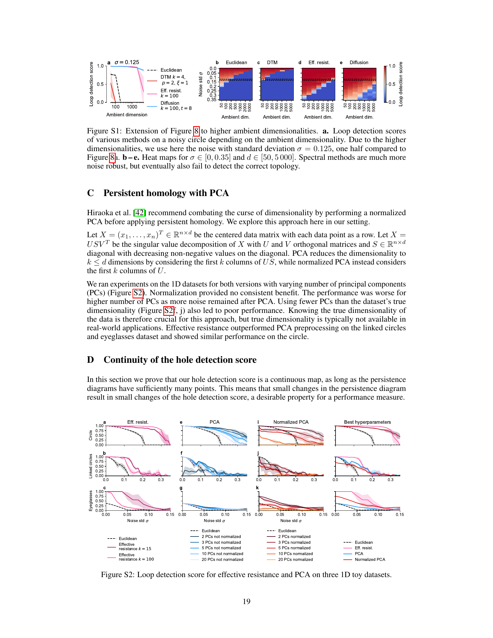
🔼 This figure demonstrates the effect of ambient dimensionality on the performance of different distance measures used in persistent homology for detecting loops in noisy data. Panel (a) shows a line graph illustrating loop detection scores for various methods at a fixed noise level (σ = 0.25) across different ambient dimensions (d). Panels (b-e) provide heatmaps that visualize loop detection scores across a range of both noise levels (σ) and ambient dimensions (d) for Euclidean distance, DTM distance, effective resistance, and diffusion distance, respectively. The heatmaps clearly show how traditional persistent homology (using Euclidean distance) becomes increasingly unreliable in higher-dimensional spaces, while the spectral methods (effective resistance and diffusion distance) are much more robust.
read the caption
Figure 8: a. Loop detection score of various methods on a noisy circle depending on the ambient dimensionality. Noise σ = 0.25. b-e. Heat maps for σ∈ [0,0.35] and d∈ [2, 50].

🔼 This figure shows the results of applying four different methods (correlation distance, DTM, effective resistance, and diffusion distance) to the Malaria dataset for detecting persistent loops. The top row displays the representative loops found by each method, overlaid on a UMAP embedding of the data. The bottom row shows the corresponding persistence diagrams. The figure highlights that spectral methods (effective resistance and diffusion distance) successfully identified the two biologically relevant loops, unlike correlation distance and DTM, which failed to accurately represent the topology.
read the caption
Figure 9: Malaria dataset. a-d. Representatives of the two most persistent loops overlaid on UMAP embedding (top) and persistence diagrams (bottom) using four methods. Biology dictates that there should be two loops (in warm colors and in cold colors) connected as in a figure eight.

🔼 This figure compares the performance of various distance metrics (Euclidean distance, Fermat distance, DTM, t-SNE, UMAP, effective resistance, diffusion distance, Laplacian Eigenmaps) for detecting cell cycle loops in six different single-cell RNA sequencing (scRNA-seq) datasets. The datasets represent various cell types (Malaria, Neurosphere, Hippocampus, Neural IPCs, HeLa2, Pancreas) with varying dimensionality (10D to 5156D). Each bar represents the detection score, indicating the success rate of identifying the true number of cell cycle loops. The hatched bars highlight cases where the most persistent loop detected did not accurately reflect the true biological cell cycle, indicating that the distance metric failed to correctly capture the underlying topology of the scRNA-seq data.
read the caption
Figure 10: Loop detection scores on six high-dimensional scRNA-seq datasets. Hatched bars indicate implausible representatives. See Figure S34 for detection scores for different hyperparameter values. Recommended methods in bold.

🔼 This figure shows how different methods perform on a noisy circle in various ambient dimensions, with varying noise levels. Panel (a) is a line graph showing the loop detection score for several methods at a fixed noise level (σ = 0.25) across different ambient dimensions (d). Panels (b-e) are heatmaps that visualize the loop detection score across a range of noise levels (σ) and ambient dimensions (d) for each method. The heatmaps help to show how robust each method is to changes in both noise and dimensionality.
read the caption
Figure 8: a. Loop detection score of various methods on a noisy circle depending on the ambient dimensionality. Noise σ = 0.25. b-e. Heat maps for σ∈ [0,0.35] and d∈ [2, 50].

🔼 The figure compares the performance of effective resistance and PCA with different numbers of principal components (PCs) for three different 1D datasets (circle, linked circles, and eyeglasses). The results demonstrate the robustness of effective resistance, even with varying hyperparameters, in comparison to PCA methods whose effectiveness depends heavily on choosing the appropriate number of PCs, knowledge not typically available in real-world applications. Noise robustness is also a key theme, with effective resistance demonstrating superiority.
read the caption
Figure S2: Loop detection score for effective resistance and PCA on three 1D toy datasets.
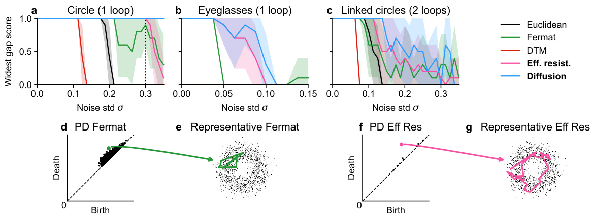
🔼 This figure compares various distance metrics used in persistent homology to detect loops in noisy high-dimensional data. The x-axis represents the standard deviation (noise level) of added Gaussian noise, and the y-axis represents a loop detection score, which measures the prominence of the detected loop. The figure shows that spectral distances (effective resistance and diffusion distance) significantly outperform other distance metrics in detecting the loop, especially in noisier settings. The results suggest that spectral distances are more robust to noise in high-dimensional spaces.
read the caption
Figure 6: Loop detection score for persistent homology with various distances on a noisy circle in R50. The best hyperparameter setting for each distance is shown. Methods are grouped into panels for visual clarity. Recommended methods in bold.
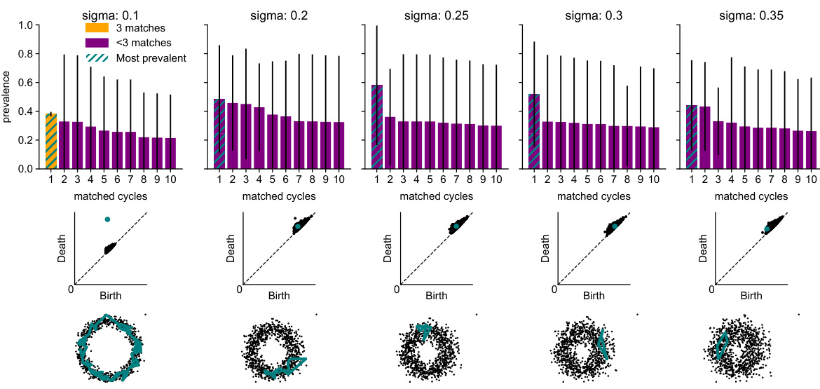
🔼 This figure shows the results of cycle matching using Euclidean distance on a noisy circle embedded in 50 dimensions with varying noise levels. The top row displays the prevalences of the 10 most persistent cycles found for each noise level, indicating how frequently a particular cycle was detected across three independent trials. The middle row shows the corresponding persistence diagrams, highlighting the most persistent features (cycles). The bottom row provides visualizations of the most prevalent cycle, overlaid on a 2-dimensional principal component analysis (PCA) of the data. The figure demonstrates how the prevalence and persistence of cycles change with increasing noise, indicating the robustness or lack thereof of the Euclidean distance in detecting the true underlying topology of the noisy data.
read the caption
Figure S4: Results for cycle matching with the Euclidean distance on a noisy circle in R50 with noise level σ. Top row: Prevalences of the 10 most prevalent cycles. Means and standard deviation over three seeds. Color indicates whether the cycle was matched for all three random seeds or not. Second row: Persistence diagrams with the most prevalent features highlighted. Third row: Representative of the most prevalent feature overlaid on a 2D PCA of the data.

🔼 This figure shows the results of cycle matching using the Euclidean distance on a noisy circle dataset in a 50-dimensional space with varying noise levels (σ). The top row displays the prevalence of the top 10 most prevalent cycles, showing the average prevalence and standard deviation across three random seeds. The color-coding indicates whether a given cycle was matched consistently across all three seeds or not. The second row presents persistence diagrams corresponding to each noise level, highlighting the most persistent features. The bottom row provides a visualization of the representative cycles from the most prevalent feature overlaid on a 2D PCA (Principal Component Analysis) of the dataset.
read the caption
Figure S4: Results for cycle matching with the Euclidean distance on a noisy circle in R50 with noise level σ. Top row: Prevalences of the 10 most prevalent cycles. Means and standard deviation over three seeds. Color indicates whether the cycle was matched for all three random seeds or not. Second row: Persistence diagrams with the most prevalent features highlighted. Third row: Representative of the most prevalent feature overlaid on a 2D PCA of the data.

🔼 The figure shows two graphs that serve as counterexamples for Proposition F.3 in the paper. The proposition states that the corrected version of effective resistance and diffusion distances are not proper metrics. The left graph demonstrates that neither corrected effective resistance nor diffusion distances between distinct points are necessarily positive, while the right graph demonstrates that corrected effective resistance does not always satisfy the triangle inequality.
read the caption
Figure S6: Counterexample graphs for Proposition F.3
🔼 This figure shows the performance of several distance metrics in persistent homology for detecting a loop structure in a noisy circle embedded in high-dimensional space. The x-axis represents the ambient dimensionality (d), ranging from 2 to 50. The y-axis represents the loop detection score. Panel (a) shows the loop detection scores for a noise standard deviation of σ = 0.25, comparing Euclidean distance, DTM (distance-to-measure), effective resistance, and diffusion distance. Panels (b) through (e) show heatmaps that visualize the loop detection scores as a function of both ambient dimensionality and noise standard deviation (σ). The heatmaps provide a more complete picture of the performance of each method across a range of conditions. The results illustrate that spectral distances (effective resistance and diffusion distance) are more robust to the curse of dimensionality than Euclidean distance, maintaining better loop detection performance even at high dimensionality and noise levels.
read the caption
Figure 8: a. Loop detection score of various methods on a noisy circle depending on the ambient dimensionality. Noise σ = 0.25. b-e. Heat maps for σ∈ [0,0.35] and d∈ [2, 50].

🔼 This figure compares the performance of different distance metrics in detecting a loop structure within a noisy dataset embedded in a 50-dimensional space. The x-axis represents the standard deviation of added Gaussian noise, while the y-axis shows the loop detection score for each distance metric. The higher the score, the better the method is at detecting the loop despite the noise. The figure showcases that spectral distances (e.g., effective resistance and diffusion distance) are significantly more robust to noise than other distance metrics, such as Euclidean distance, Fermat distance, geodesic distance, and distance-to-measure. The recommended methods are highlighted in bold.
read the caption
Figure 6: Loop detection score for persistent homology with various distances on a noisy circle in R50. The best hyperparameter setting for each distance is shown. Methods are grouped into panels for visual clarity. Recommended methods in bold.
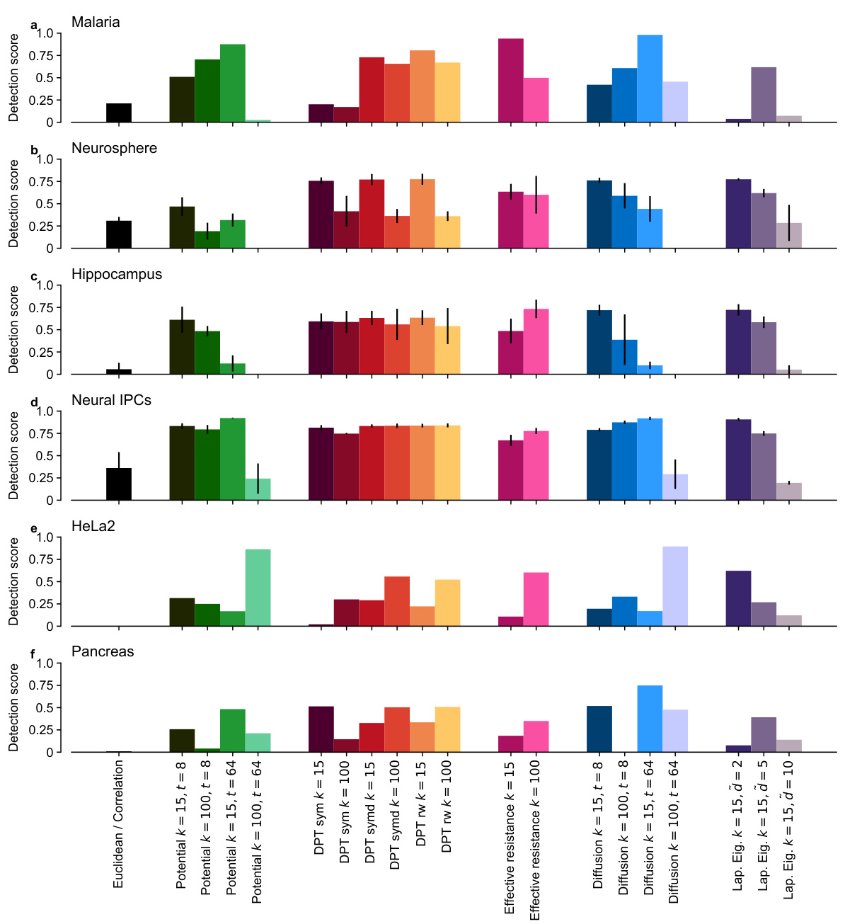
🔼 This figure shows the loop detection scores for six different high-dimensional single-cell RNA sequencing datasets. Various distance metrics were used as input to persistent homology to identify topological loops within the data. The figure highlights the performance of different methods, emphasizing the superior performance of spectral methods (shown in bold). Hatched bars indicate instances where the most persistent loop identified by a method was deemed implausible upon visual inspection. Figure S34 provides additional detail on the detection scores for different hyperparameter values.
read the caption
Figure 10: Loop detection scores on six high-dimensional scRNA-seq datasets. Hatched bars indicate implausible representatives. See Figure S34 for detection scores for different hyperparameter values. Recommended methods in bold.
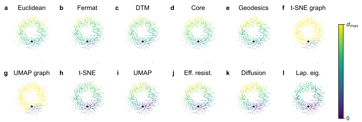
🔼 This figure visualizes different distance metrics applied to a noisy circle dataset in 50 dimensions. Each subfigure represents a different distance metric (Euclidean, Fermat, DTM, Core, Geodesics, t-SNE graph, UMAP graph, t-SNE, UMAP, Effective Resistance, Diffusion, and Laplacian Eigenmaps). The data is projected to 2D using PCA, and color-coding shows the distance from a single, highlighted data point. This allows for a visual comparison of how each distance metric captures the underlying structure of the data despite the noise.
read the caption
Figure S10: Visualization of all distances on the noisy circle in R50 with σ = 0.25. All scatter plots are the 2D PCA of the 50D dataset. The colors indicate the distance to the highlighted point.
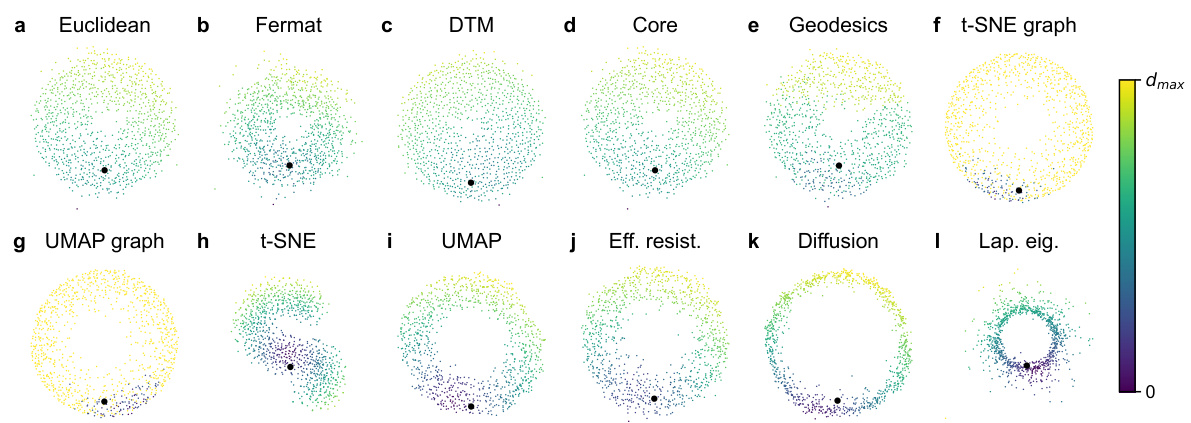
🔼 This figure visualizes different distance metrics applied to a noisy circle embedded in 50-dimensional space. Each subplot shows a 2D principal component analysis (PCA) projection of the data, colored according to the distance from a highlighted point. The distances shown include Euclidean, Fermat, DTM, core distance, geodesic distance, t-SNE graph affinities, UMAP graph affinities, t-SNE embedding distances, UMAP embedding distances, effective resistance, diffusion distance, and Laplacian Eigenmaps distances. This allows for a visual comparison of how each metric captures the structure of the noisy circle, highlighting the relative robustness of each method to high-dimensional noise.
read the caption
Figure S10: Visualization of all distances on the noisy circle in R50 with σ = 0.25. All scatter plots are the 2D PCA of the 50D dataset. The colors indicate the distance to the highlighted point.

🔼 This figure shows a comparison of different methods for detecting topological loops in noisy high-dimensional data. Panel (a) displays a 2D PCA of a noisy circle embedded in 50 dimensions, with representative loops overlaid. Panel (b) compares persistence diagrams using Euclidean distance and effective resistance to visualize the loops. Panel (c) shows the loop detection scores for both distances. Finally, panels (d) and (e) show the UMAP and t-SNE embeddings, which are dimensionality reduction techniques, illustrating the loop structure in 2D.
read the caption
Figure 1: a. 2D PCA of a noisy circle (σ = 0.25, radius 1) in R50. Overlaid are representative cycles of the most persistent loops. b. Persistence diagrams using Euclidean distance and the effective resistance. c. Loop detection scores of persistent homology using effective resistance and Euclidean distance. d, e. UMAP and t-SNE embeddings of the same data, showing the loop structure in 2D.

🔼 This figure shows the effect of adding Gaussian noise with different standard deviations (σ) to a dataset of points sampled from a circle. The top row (a-i) displays the data in its original 2-dimensional space, while the bottom row (j-q) shows the result of applying multidimensional scaling (MDS) to the Euclidean distances between the points in a 50-dimensional space. As the noise level (σ) increases, the circular structure of the data becomes less apparent in the 50-dimensional MDS representation, demonstrating the effect of high-dimensional noise on the Euclidean distance metric.
read the caption
Figure S13: Circle with Gaussian noise of different standard deviation σ. a-i. Original data in ambient dimension d = 2. j-q. Multidimensional scaling of the Euclidean distance of the data in ambient dimension d = 50.

🔼 This figure shows the 2D embeddings of six different single-cell RNA sequencing datasets. The Malaria and Neural IPC datasets are visualized using UMAP embeddings, while the Neurosphere, Hippocampus, HeLa2, and Pancreas datasets are visualized using a 2D linear projection designed to highlight the cell cycle. Each plot shows the distribution of cells in the 2D embedding space, with different colors representing different cell types or cell cycle phases.
read the caption
Figure S14: 2D embeddings of all six single-cell datasets. a, f. UMAP embeddings of the Malaria [43] and the Neural IPC datasets [8]. We recomputed the embedding for the Malaria dataset using UMAP hyperparameters provided in the original publication, and subsetted an author-provided UMAP of a superset of telencephalic exitatory cells to the Neural IPC. The text legend refers to Malaria cell types. b-e. 2D linear projection constructed to bring out the cell cycle ('tricycle embedding') [89] of the Neurosphere, Hippocampus, HeLa2, and Pancreas datasets. We used the projection coordinates provided by Zheng et al. [89].

🔼 This figure expands on Figure 8 by investigating the performance of various methods on higher ambient dimensionalities. The loop detection scores are plotted against the noise level and ambient dimension, showing that spectral methods are more robust than other methods, but eventually fail to detect the correct topology as both noise level and dimensionality increase. Heatmaps show the performance of various distances in the presence of increasing levels of noise across a range of ambient dimensions from 50 to 5000.
read the caption
Figure S1: Extension of Figure 8 to higher ambient dimensionalities. a. Loop detection scores of various methods on a noisy circle depending on the ambient dimensionality. Due to the higher dimensionalities, we use here the noise with standard deviation σ = 0.125, one half compared to Figure 8a. b-e. Heat maps for σ∈ [0, 0.35] and d ∈ [50, 5000]. Spectral methods are much more noise robust, but eventually also fail to detect the correct topology.
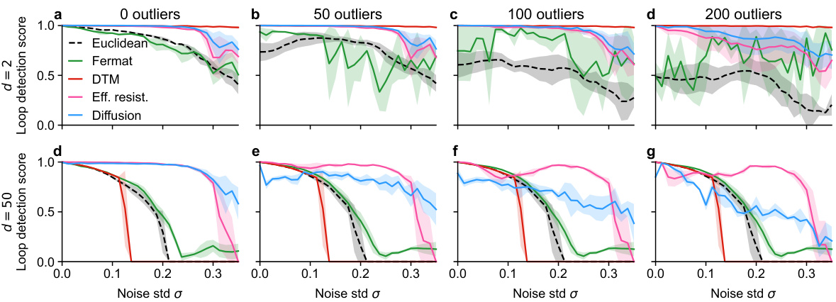
🔼 This figure compares the performance of different distance metrics in persistent homology on a noisy circle dataset with added outliers in low (d=2) and high (d=50) dimensional ambient spaces. The results show that spectral methods (effective resistance and diffusion distance) are more robust to outliers than Euclidean distance, Fermat distance, and DTM. In high dimensions, outliers have less impact due to the increased sparsity.
read the caption
Figure S16: Loop detection performance of various methods on the noisy circle in the presence of outliers in low- and high-dimensional ambient space. Outliers were sampled uniformly from an axis-aligned cube around the data. a-d. In low ambient dimension (d = 2) adding outliers hurt the performance of the Euclidean and Fermat distances, but barely affected the performance of the spectral methods and not at all DTM's excellent performance. e-g. In high ambient dimensionality (d = 50) outliers did not further decrease the weak performance of non-spectral methods. Diffusion distance was somewhat outlier-sensitive, but could still detect the loop structure in the high Gaussian noise setting. Effective resistance performed best overall and was not very outlier-sensitive.

🔼 This figure shows the performance of several distance metrics, when combined with persistent homology, for detecting loops in a noisy circle embedded in a high-dimensional space (R50). Different methods are compared based on a ’loop detection score’, which measures the prominence of the true loop in the persistence diagrams. The scores are plotted against the standard deviation of the added Gaussian noise. The figure highlights that spectral distances (effective resistance and diffusion distance) are particularly robust to high-dimensional noise compared to Euclidean distance and other methods (Fermat, DTM, core distance, geodesic distance on kNN graph, UMAP/t-SNE graph, UMAP/t-SNE embeddings).
read the caption
Figure 6: Loop detection score for persistent homology with various distances on a noisy circle in R50. The best hyperparameter setting for each distance is shown. Methods are grouped into panels for visual clarity. Recommended methods in bold.

🔼 This figure compares different methods for detecting topological structures in noisy high-dimensional data. Panel (a) shows a 2D PCA projection of a noisy circle embedded in 50 dimensions, with representative cycles from persistent homology overlaid. Panel (b) shows persistence diagrams for both Euclidean distance and effective resistance. Panel (c) shows loop detection scores, comparing effective resistance and Euclidean distance. Panels (d) and (e) demonstrate the ability of UMAP and t-SNE to reveal the underlying loop structure in 2D.
read the caption
Figure 1: a. 2D PCA of a noisy circle (σ = 0.25, radius 1) in R50. Overlaid are representative cycles of the most persistent loops. b. Persistence diagrams using Euclidean distance and the effective resistance. c. Loop detection scores of persistent homology using effective resistance and Euclidean distance. d, e. UMAP and t-SNE embeddings of the same data, showing the loop structure in 2D.

🔼 This figure presents a comparison of different distance metrics used in persistent homology for detecting cell cycle loops in high-dimensional single-cell RNA sequencing data. Six datasets from different biological sources are used. The loop detection score measures the performance of each method in identifying the correct number of loops. Spectral methods (effective resistance, diffusion distance, Laplacian Eigenmaps) consistently outperformed alternative approaches, and especially effective resistance delivered high scores with biologically plausible loop representatives.
read the caption
Figure 10: Loop detection scores on six high-dimensional scRNA-seq datasets. Hatched bars indicate implausible representatives. See Figure S34 for detection scores for different hyperparameter values. Recommended methods in bold.

🔼 This figure compares several versions of effective resistance to the Euclidean distance in detecting loops on a noisy circle in 50-dimensional space. The versions of effective resistance considered include using a weighted or unweighted k-nearest neighbor (kNN) graph, and taking the square root of the effective resistance. The results show that there is little difference in performance between these versions, and they all significantly outperform the Euclidean distance across all noise levels. Only the uncorrected (naive) version of effective resistance performs poorly.
read the caption
Figure S20: Loop detection score on noisy S¹ C R50 for various versions of effective resistance. There was little difference between using the weighted kNN graph, unweighted kNN graph, and using the square root of effective resistance based on the unweighted kNN graph. The latter got filtered out for high noise levels. Using k = 100 instead of k = 15 helped only marginally in this dataset. The uncorrected (naive) version of effective resistance collapsed already at very small noise levels.

🔼 This figure demonstrates the failure of traditional persistent homology with Euclidean distance to detect the topology of a noisy circle in a high-dimensional space. Panel (a) shows a 2D PCA of the data, with representative cycles of the most persistent loops overlaid. Panel (b) presents persistence diagrams using both Euclidean distance and effective resistance. Panel (c) shows the loop detection scores, highlighting the superior performance of effective resistance. Finally, Panels (d) and (e) illustrate that dimensionality reduction techniques like UMAP and t-SNE can successfully reveal the loop structure in 2D.
read the caption
Figure 1: a. 2D PCA of a noisy circle (σ = 0.25, radius 1) in R50. Overlaid are representative cycles of the most persistent loops. b. Persistence diagrams using Euclidean distance and the effective resistance. c. Loop detection scores of persistent homology using effective resistance and Euclidean distance. d, e. UMAP and t-SNE embeddings of the same data, showing the loop structure in 2D.
🔼 This figure compares different methods for detecting topological features (loops) in noisy high-dimensional data. Panel (a) shows a 2D PCA projection of a noisy circle embedded in 50 dimensions, with representative cycles from persistent homology highlighted. Panel (b) shows persistence diagrams, which plot the ‘birth’ and ‘death’ times of topological features, using both Euclidean distance and a spectral distance called ’effective resistance’. Panel (c) quantifies the ability of each distance metric to correctly identify the loop by computing a ’loop detection score’. Panels (d) and (e) show the same data visualized with UMAP and t-SNE, demonstrating that spectral methods can accurately reveal the underlying loop structure even in the presence of significant noise.
read the caption
Figure 1: a. 2D PCA of a noisy circle (σ = 0.25, radius 1) in R50. Overlaid are representative cycles of the most persistent loops. b. Persistence diagrams using Euclidean distance and the effective resistance. c. Loop detection scores of persistent homology using effective resistance and Euclidean distance. d, e. UMAP and t-SNE embeddings of the same data, showing the loop structure in 2D.

🔼 This figure shows the performance of various distance metrics used in persistent homology for detecting loops in a noisy circle dataset embedded in 50-dimensional space. The x-axis represents the standard deviation of added Gaussian noise, and the y-axis represents the loop detection score, a metric indicating the accuracy of loop detection. The figure is divided into panels, each showing a group of related methods (Euclidean distance, Fermat distances, Distance-to-measure, core distances, geodesics distances, UMAP graph distances, t-SNE graph distances, UMAP embeddings, t-SNE embeddings, effective resistance distances, diffusion distances, Laplacian eigenmaps distances). The results indicate that spectral distances (effective resistance and diffusion distance) significantly outperform other methods in robustness to high-dimensional noise.
read the caption
Figure 6: Loop detection score for persistent homology with various distances on a noisy circle in R50. The best hyperparameter setting for each distance is shown. Methods are grouped into panels for visual clarity. Recommended methods in bold.

🔼 This figure presents the loop detection scores for various distances used in persistent homology on a noisy circle in 50-dimensional space. The x-axis represents the noise standard deviation (σ), and the y-axis shows the loop detection score. Each line represents a different distance metric, with the best hyperparameters used for each. The methods are grouped into panels to improve clarity. The recommended methods, which achieved the best performance, are highlighted in bold. This figure demonstrates the effectiveness of different distance metrics when used with persistent homology to detect topological features (loops) in high-dimensional, noisy data.
read the caption
Figure 6: Loop detection score for persistent homology with various distances on a noisy circle in R50. The best hyperparameter setting for each distance is shown. Methods are grouped into panels for visual clarity. Recommended methods in bold.

🔼 This figure displays the loop detection score for persistent homology using different distance metrics on a noisy circle dataset embedded in 50-dimensional space. The x-axis represents the standard deviation (noise level) of the added Gaussian noise. The y-axis shows the loop detection score, a metric indicating how well persistent homology identifies the loop structure amidst noise. Each line represents a different distance metric, categorized into panels for clarity: Euclidean, Fermat, Distance-to-Measure (DTM), Geodesics, UMAP graph, t-SNE graph, UMAP, t-SNE, Effective resistance, and Diffusion. The bold lines highlight the methods that performed best according to the authors.
read the caption
Figure 6: Loop detection score for persistent homology with various distances on a noisy circle in R50. The best hyperparameter setting for each distance is shown. Methods are grouped into panels for visual clarity. Recommended methods in bold.

🔼 This figure compares the performance of different distance metrics on a noisy circle embedded in 50-dimensional space. The loop detection score measures how well persistent homology identifies the correct loop structure using various distances. The figure shows that spectral distances (effective resistance and diffusion distance) significantly outperform other distances in detecting the loop structure, even in the presence of high-dimensional noise. The results highlight the robustness of spectral distances to noise and their effectiveness in capturing the topological structure of the data.
read the caption
Figure 6: Loop detection score for persistent homology with various distances on a noisy circle in R50. The best hyperparameter setting for each distance is shown. Methods are grouped into panels for visual clarity. Recommended methods in bold.

🔼 This figure displays the loop detection scores for persistent homology using various distances on a noisy circle embedded in a 50-dimensional space. The x-axis represents the standard deviation (noise level) of the added Gaussian noise, and the y-axis shows the loop detection score. Different methods for calculating distance metrics are compared, grouped into panels (Euclidean, Fermat, DTM, etc.), and the optimal hyperparameters for each method are used. The goal is to evaluate which distance metric is most robust to noise in high-dimensional data for detecting topological features.
read the caption
Figure 6: Loop detection score for persistent homology with various distances on a noisy circle in R50. The best hyperparameter setting for each distance is shown. Methods are grouped into panels for visual clarity. Recommended methods in bold.
🔼 This figure compares the performance of several distance metrics in detecting loops in a noisy circle embedded in 50-dimensional space. Each point represents the loop detection score, calculated using persistent homology for a given distance metric and noise level. The hyperparameters for each distance metric were optimized to achieve the best performance for the task. Euclidean distance shows poor performance at higher noise levels, while spectral distances (effective resistance, diffusion distances, and Laplacian Eigenmaps) consistently show superior performance. The results highlight the advantage of spectral distances over traditional Euclidean distance for topological data analysis in high-dimensional noisy data.
read the caption
Figure 6: Loop detection score for persistent homology with various distances on a noisy circle in R50. The best hyperparameter setting for each distance is shown. Methods are grouped into panels for visual clarity. Recommended methods in bold.

🔼 This figure demonstrates the limitations of traditional persistent homology when dealing with high-dimensional noisy data. Panel (a) shows a 2D PCA of a noisy circle embedded in a 50-dimensional space, along with representative cycles of the most persistent loops identified by persistent homology using Euclidean distance. Panel (b) compares persistence diagrams using Euclidean distance and the effective resistance as distance metrics, highlighting the failure of Euclidean distance to detect the true loop. Panel (c) further quantifies the difference in loop detection scores between Euclidean distance and effective resistance, illustrating the improved robustness of effective resistance to noise. Finally, panels (d) and (e) visualize the same data using UMAP and t-SNE, respectively, which successfully recover the underlying circular structure.
read the caption
Figure 1: a. 2D PCA of a noisy circle (σ = 0.25, radius 1) in R50. Overlaid are representative cycles of the most persistent loops. b. Persistence diagrams using Euclidean distance and the effective resistance. c. Loop detection scores of persistent homology using effective resistance and Euclidean distance. d, e. UMAP and t-SNE embeddings of the same data, showing the loop structure in 2D.

🔼 The figure shows the loop detection score for persistent homology using different distance measures on a noisy circle in a 50-dimensional space. The x-axis represents the noise standard deviation (σ), and the y-axis represents the loop detection score. Different distance measures are grouped into panels (Euclidean, Fermat, DTM, Core, Geodesics, UMAP graph, t-SNE graph, UMAP, t-SNE, Effective resistance, Diffusion, Laplacian Eig.). Each panel shows the performance of various methods with their best hyperparameter settings. The recommended methods are highlighted in bold.
read the caption
Figure 6: Loop detection score for persistent homology with various distances on a noisy circle in R50. The best hyperparameter setting for each distance is shown. Methods are grouped into panels for visual clarity. Recommended methods in bold.

🔼 This figure shows the result of applying persistent homology with different distance metrics to a noisy torus dataset. The experiment is conducted twice with different sample sizes (n=1000 and n=5000) to examine how the performance of each distance metric changes with increasing data density. Spectral methods (effective resistance and diffusion distance) exhibit a substantial performance improvement with the larger dataset (n=5000), while the difference is less pronounced for other distance metrics (Euclidean, Fermat, and DTM). This highlights the effectiveness of spectral methods in capturing topological features, especially when the data density is sufficient.
read the caption
Figure S31: 2-loop detection score for persistent homology with various distances on a noisy torus with different sample size n. For more points, all methods performed better as the shape of the torus gets sampled more densely. The difference in performance is particularly striking for the spectral methods which outperformed the others for n = 5000 points, but did not for n = 1000.

🔼 This figure analyzes why diffusion distances fail on the torus dataset with 1000 data points. It shows that the eigenvalue decay of diffusion distances with t=8 and t=64 suppresses the relevant eigenvectors, unlike effective resistance and diffusion distances with t=2. Eigenvector analysis reveals that the loops along and around the torus are encoded in specific eigenvectors. This explains why diffusion distances, which rely on random walks, struggle to capture the torus’s topology effectively.
read the caption
Figure S32: Diffusion distances failed on the torus with n = 1000 because its eigenvalue decay suppressed the relevant eigenvectors. a. 2-loop detection score for the torus in d = 50 ambient dimensions. Diffusion distances with t = 2 diffusion steps were on par with effective resistance and Euclidean distance. b. Decay of eigenvalues in various spectral distances on the noiseless torus. Diffusion distances with t = 8, 64 only had contribution below 0.1 for the fifth and sixth eigenvectors, while effective resistance and diffusion distance with t = 2 had substantial contributions from the first ~10 eigenvectors. c-f. Eigenvectors of the symmetric graph Laplacian of a symmetric 100-nearest-neighbor graph of the noiseless torus. Coordinates are the angles of each point along ($\[phi]\]$) and around ($\[\theta]\]$) the tube of the torus. The loop along the tube is encoded in the first two eigenvectors, the loop around the tube in the fifth and sixth eigenvectors.
🔼 This figure compares the performance of different distance metrics used in persistent homology for detecting a loop in a noisy high-dimensional dataset. The x-axis represents the standard deviation (noise level) of the added Gaussian noise. The y-axis represents the loop detection score, a metric indicating the accuracy of loop detection. Different distance metrics (Euclidean, Fermat, DTM, core distance, geodesic distances on kNN graphs, UMAP graph distances, t-SNE graph distances, UMAP embeddings, t-SNE embeddings, effective resistance, diffusion distance, Laplacian Eigenmaps) are tested with various hyperparameter settings. The results show that spectral distances (effective resistance and diffusion distance) significantly outperform other methods, especially at higher noise levels.
read the caption
Figure 6: Loop detection score for persistent homology with various distances on a noisy circle in R50. The best hyperparameter setting for each distance is shown. Methods are grouped into panels for visual clarity. Recommended methods in bold.

🔼 This figure shows the loop detection scores for six different high-dimensional single-cell RNA sequencing datasets. The scores are obtained using various distance measures within the context of persistent homology, and the performance of different methods is compared. The use of spectral methods (shown in bold) for persistent homology is highlighted as these methods consistently perform well across various datasets and are more robust to noise in high-dimensional data compared to other methods.
read the caption
Figure 10: Loop detection scores on six high-dimensional scRNA-seq datasets. Hatched bars indicate implausible representatives. See Figure S34 for detection scores for different hyperparameter values. Recommended methods in bold.
More on tables
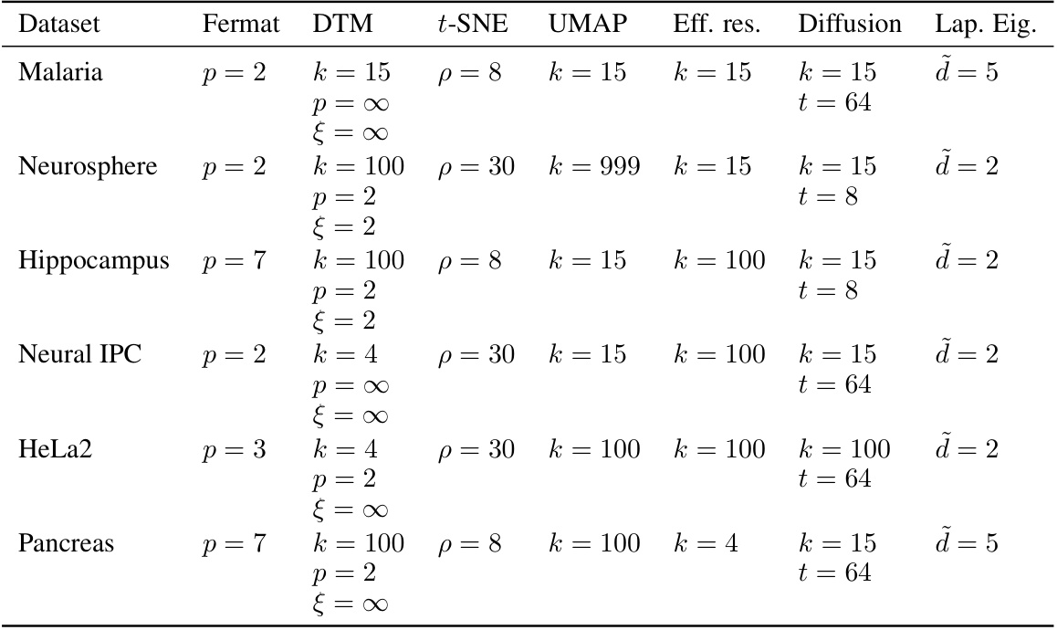
🔼 This table lists the best hyperparameter settings used for each distance metric in the single-cell RNA sequencing data analysis shown in Figure 10 of the paper. The hyperparameters were chosen based on maximizing the loop detection score, as described in the paper. The table is organized by dataset, and the hyperparameters for the Fermat distance, DTM distance, t-SNE affinities, UMAP affinities, effective resistance, diffusion distance, and Laplacian Eigenmaps are given. Note that no hyperparameter settings for DTM passed the thresholding.
read the caption
Table S2: The optimal hyperparameters that were selected in Figure 10. For DTM we report the best setting without thresholding (because none of the DTM runs passed our birth/death thresholding, so all sm scores for all parameter combinations are zero).

🔼 This table shows the best hyperparameter settings for different distance metrics used in the persistent homology analysis in Figure 7 of the paper. The hyperparameters were selected to maximize the performance of the methods on the datasets. Note that the torus and sphere datasets were analysed separately for loop detection (H1) and void detection (H2) tasks, resulting in different optimal settings for each task.
read the caption
Table S1: The optimal hyperparameters that were selected in Figure 7. For torus and sphere, we consider the case of loop detection (H1) and void detection (H2) separately.

🔼 This table shows the optimal hyperparameter settings used for different distance measures in Figure S16 of the paper. The figure shows the loop detection performance of various methods on a noisy circle in the presence of outliers in both low- and high-dimensional ambient spaces. The hyperparameters were selected to maximize the area under the curve of the loop detection score. The table lists hyperparameters for different distance measures, including Fermat, DTM, effective resistance, and diffusion distances, in different ambient dimensions and different numbers of outliers.
read the caption
Table S4: The optimal hyperparameters that were selected in Figure S16.

🔼 This table shows the time it took to compute pairwise distances and persistent homology for different datasets. The datasets include a circle, a sphere, and those with different noise levels. For each dataset, the number of data points (n), the noise level (σ), the distance used, the dimension of the topological features considered, the time for distance calculation, and the time for persistent homology calculation are given. The time is presented as mean ± standard deviation over three random seeds.
read the caption
Table S5: Exemplary run times in seconds.
Full paper#
