↗ OpenReview ↗ NeurIPS Homepage ↗ Chat
TL;DR#
Magnetic Resonance Imaging (MRI) suffers from motion artifacts due to long scan times. Correcting for this motion is crucial but challenging, particularly in 3D MRI where existing methods are slow and often inaccurate. Current approaches often rely on simulated motion data for training, which limits their generalizability. Deep learning methods offer speed improvements but most focus only on 2D in-plane motion correction.
MotionTTT addresses these issues with a novel test-time training (TTT) method. It uses a 2D reconstruction network trained on motion-free data, cleverly leveraging the network’s properties to estimate motion parameters directly from the motion-corrupted 3D data. The estimated parameters enable accurate motion correction. The method proves effective for both simulated and real motion-corrupted data, outperforming existing methods in accuracy and speed, particularly in cases of severe motion. It’s the first deep learning-based method for 3D rigid motion estimation tailored to MRI.
Key Takeaways#
Why does it matter?#
This paper is important because it introduces a novel deep learning approach for motion correction in 3D MRI, a significant challenge in medical imaging. The method’s speed and accuracy, demonstrated on both simulated and real data, make it highly relevant to researchers seeking to improve the quality and efficiency of MRI scans. It opens avenues for research into new deep learning techniques for motion estimation and correction in various medical imaging modalities.
Visual Insights#

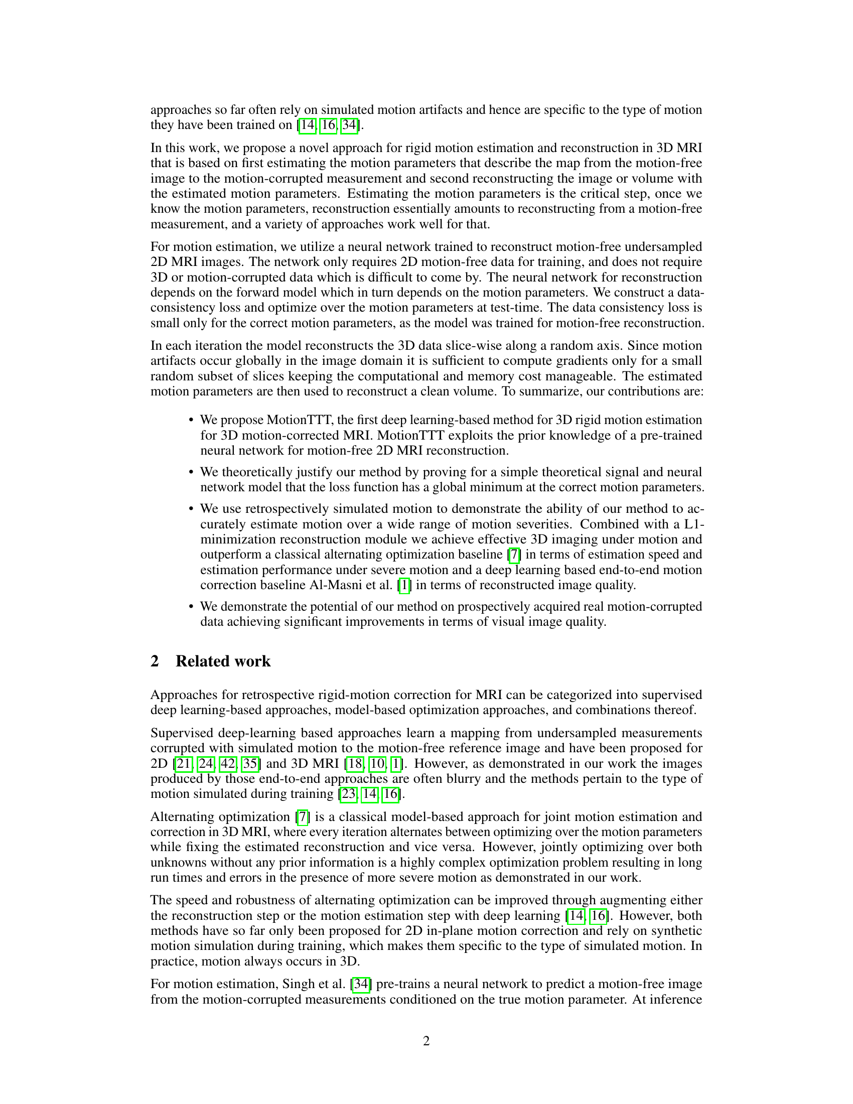
This figure displays the data used in the MotionTTT method. Panel (a) shows the magnitude of a 3D volume, and panel (b) shows its corresponding 3D k-space data. Panels (c) and (d) illustrate the undersampling masks used for simulated and real data, respectively. The color-coding in (c) and (d) represents the sampling trajectory, where each color indicates which lines along the readout dimension (kz) are sampled within the same shot (out of 50 shots). Panel (c) shows an interleaved sampling trajectory, while panel (d) shows a random sampling trajectory.

This table lists the MRI sequence parameters used for acquiring real motion-corrupted data in the experiments described in Section 6.3. The parameters include flip angle, repetition time (TR), echo time (TE), inversion time (TI), turbo factor, number of shots, and other relevant details of the acquisition. It provides a detailed technical description of the experimental setup.
In-depth insights#
MotionTTT Method#
The MotionTTT method is a novel deep learning approach for 3D motion-corrected MRI. It leverages a test-time training (TTT) strategy, using a pre-trained 2D motion-free reconstruction network. The core idea is to treat motion parameters as additional network parameters, optimizing them during testing to minimize the reconstruction loss. This is clever because a network trained on motion-free data will inherently have low loss when no motion is present. The method’s key advantage is its ability to estimate 3D rigid motion using only 2D networks, avoiding the computational burden of training on large, scarce 3D datasets. While proven effective on both simulated and real motion-corrupted data, theoretical justification is provided for a simplified model. A limitation is its reliance on pre-trained networks and potential sensitivity to the type of motion encountered. Despite this, the theoretical analysis and experimental results on prospectively collected real data show a significant improvement in visual image quality. The use of 2D networks and TTT make the method particularly appealing for its computational efficiency and applicability to clinical workflows.
3D Motion Estimation#
3D motion estimation in medical imaging, particularly MRI, presents a significant challenge due to the extended scan times. Inaccurate motion estimation leads to artifacts and misdiagnosis. Existing methods often rely on 2D approaches or simulated data, failing to capture the complexity of real-world 3D motion. This necessitates advanced techniques that can robustly estimate 3D motion from incomplete and noisy data. Deep learning methods offer potential advantages, enabling the learning of complex motion patterns from data. However, limitations exist with respect to data availability, generalizability to unseen motions, and computational cost. Test-time training (TTT) is a promising direction, allowing for adaptation to specific patient motion during reconstruction. A key aspect is the development of a loss function that effectively guides the learning process towards accurate 3D motion parameter estimation. Theoretical justification and validation are crucial to ensure that the method provably converges to the correct solution, at least under simplifying assumptions. The results are usually validated using both simulated and real motion data, quantifying the accuracy of motion estimation and improvement in image quality.
Simulated Motion#
The section on simulated motion is crucial for evaluating the MotionTTT algorithm because it allows for controlled experiments with known ground truth. Realistic motion simulation is key, and the authors use both inter-shot (motion between acquisitions) and intra-shot (motion during a single acquisition) scenarios. The use of interleaved and random sampling trajectories adds another layer of complexity and realism, testing the algorithm’s robustness to different acquisition patterns. The generation of motion parameters is also described, showing a focus on realistic movement patterns. The use of a variety of metrics, such as PSNR (Peak Signal-to-Noise Ratio), likely helps ascertain the algorithm’s accuracy. Careful attention to the various factors impacting motion simulation (number of motion events, magnitude of translations and rotations, sampling trajectory) demonstrates a rigorous approach to validation. These experiments, which include both quantitative and qualitative results, build a compelling case for the algorithm’s ability to correctly estimate and correct for motion artifacts in MRI scans. The inclusion of visual difference images is particularly helpful for understanding the algorithm’s performance in scenarios with different levels of motion severity. The simulated motion results form a strong foundation for later tests using real motion data, providing a benchmark against which to compare its performance.
Real-World Testing#
A dedicated ‘Real-World Testing’ section in a research paper would significantly strengthen its validity and impact. It should go beyond simply stating the application of the method to real-world data; instead, it needs a rigorous evaluation against established baselines, preferably including those used in simulated experiments. The section must address the challenges and limitations encountered when transitioning from simulated to real-world scenarios, such as noise, artifacts, and data variability. A qualitative analysis is crucial—visual comparisons, or detailed descriptions of performance in specific application domains, can add weight to the claims. Metrics beyond simple accuracy, such as robustness to different noise levels or computational efficiency, must be considered, along with any unexpected failures or edge-case behaviors observed in the real-world data. Finally, the authors should discuss any generalizability issues or limitations revealed by real-world data and propose future improvements. This comprehensive approach will build trust and confidence in the method’s applicability.
Future Directions#
The research paper’s ‘Future Directions’ section would ideally explore several promising avenues. Improving the reconstruction module is crucial; the current L1-minimization approach could benefit from incorporating more sophisticated deep learning methods, potentially leveraging diffusion models or other advanced techniques for superior image quality. Addressing the reliance on fully-sampled training data is another key area; investigating self-supervised learning strategies or developing methods capable of learning from undersampled data would significantly enhance the practicality and generalizability of the proposed MotionTTT framework. Extending the methodology to handle more complex motion patterns (beyond rigid-body motion) is also important for real-world applicability. Exploring non-rigid transformations or incorporating physiological motion models could enhance robustness. Finally, thorough evaluation on a wider range of MRI sequences and clinical datasets is needed to validate the generalizability of MotionTTT and establish its clinical utility. Investigating the impact of different scanner hardware, acquisition parameters, and imaging protocols on the accuracy and efficiency of the method would be particularly valuable.
More visual insights#
More on figures
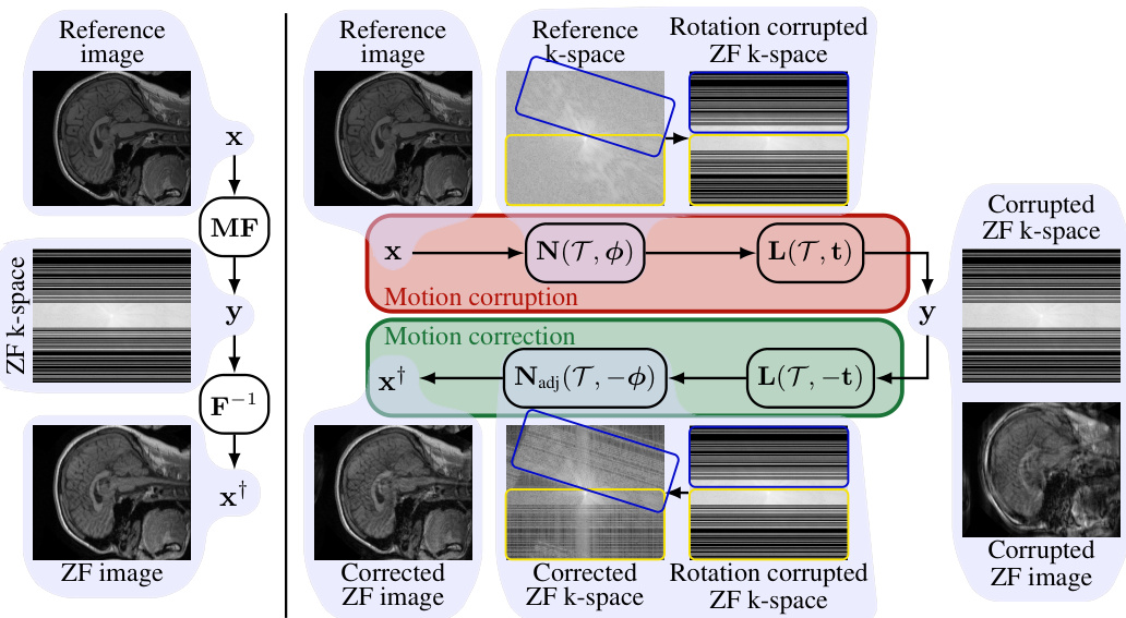
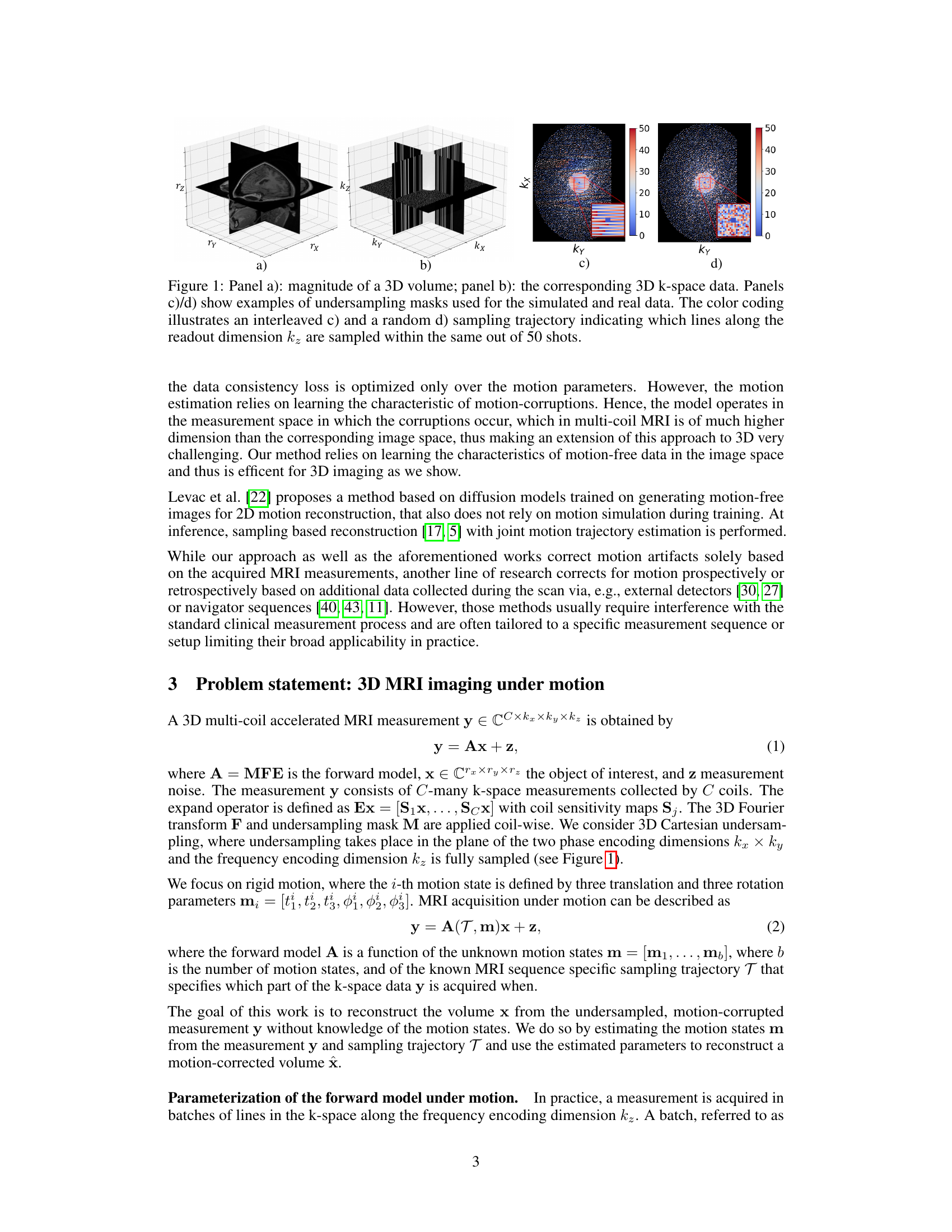
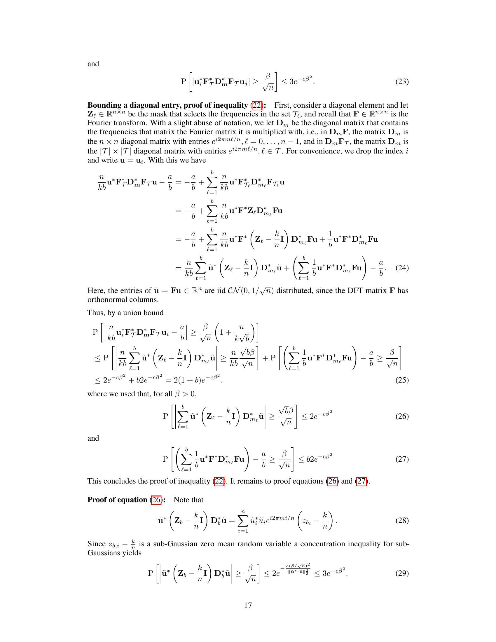
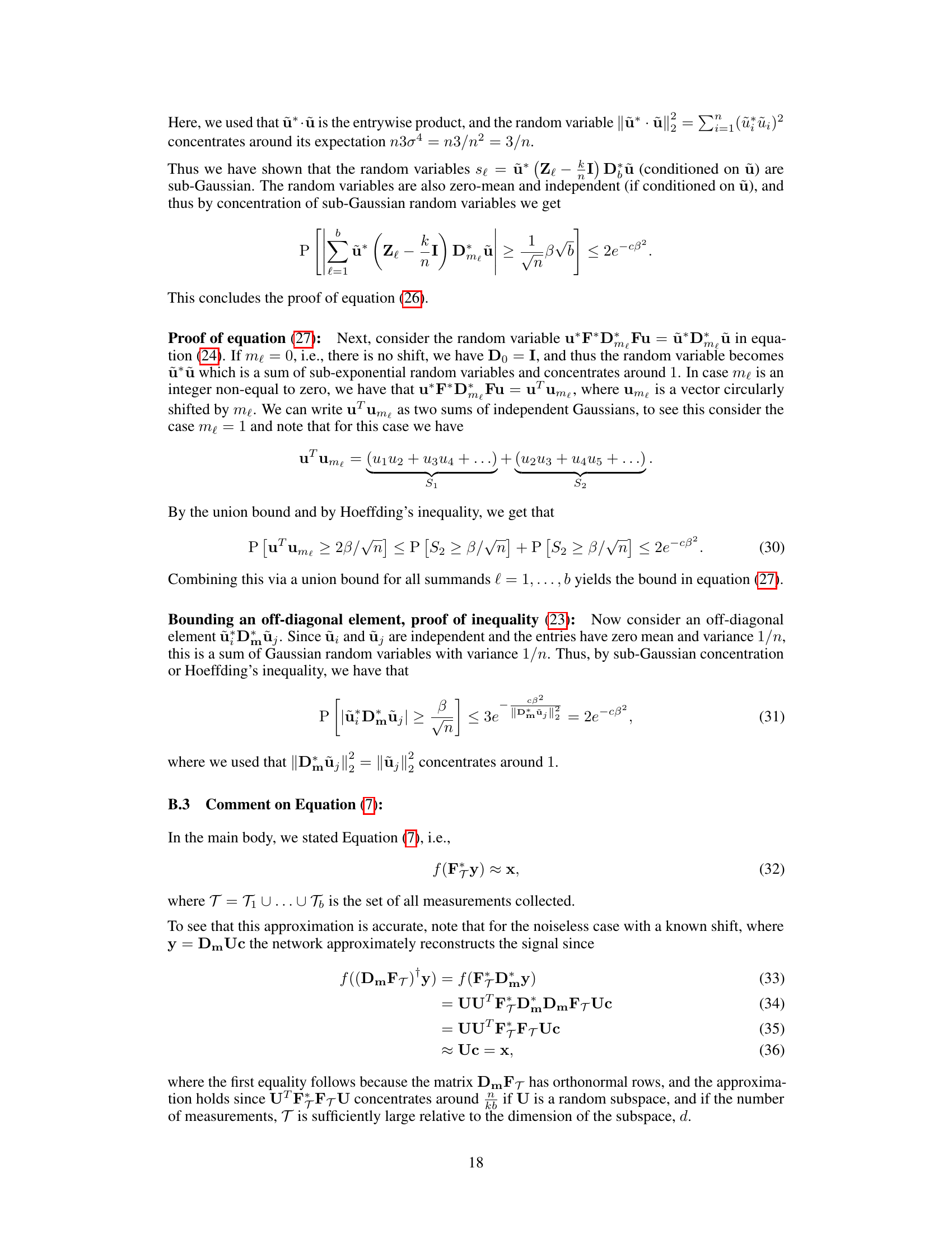
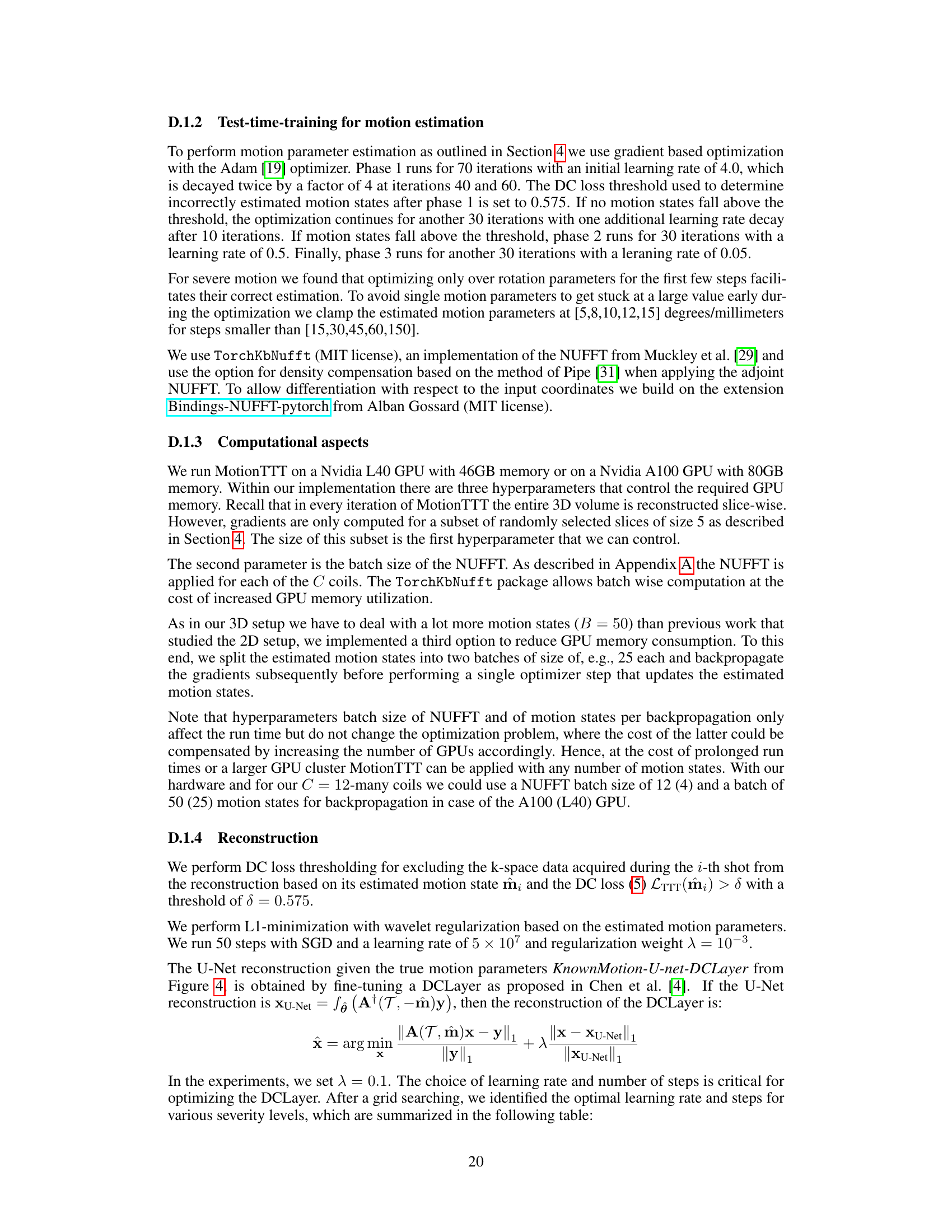
This figure illustrates the MRI forward models with and without motion for a 2D single-coil setup. The left side shows the process without motion: the reference image is transformed to k-space, undersampled, and then reconstructed using the inverse Fourier transform. The right side shows what happens with motion: rotations are applied using the non-uniform fast Fourier transform (NUFFT), and translations are implemented with linear phase shifts. This introduces artifacts into the reconstructed image, because some areas of k-space are oversampled while others are undersampled during the motion.

The figure shows the loss function for different values of the shift parameter m₁, with varying numbers of other parameters (m₂, m₃, m₄) set to values different from the true shift (m* = 0). The plot demonstrates that a sharp minimum in the loss occurs when m₁ matches the true shift, illustrating the theoretical justification for MotionTTT’s ability to estimate motion parameters.
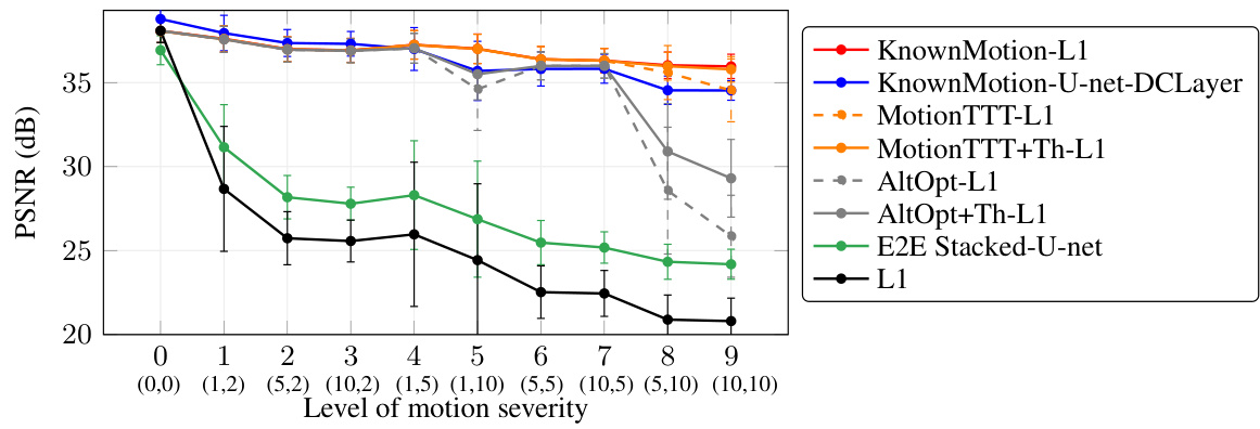
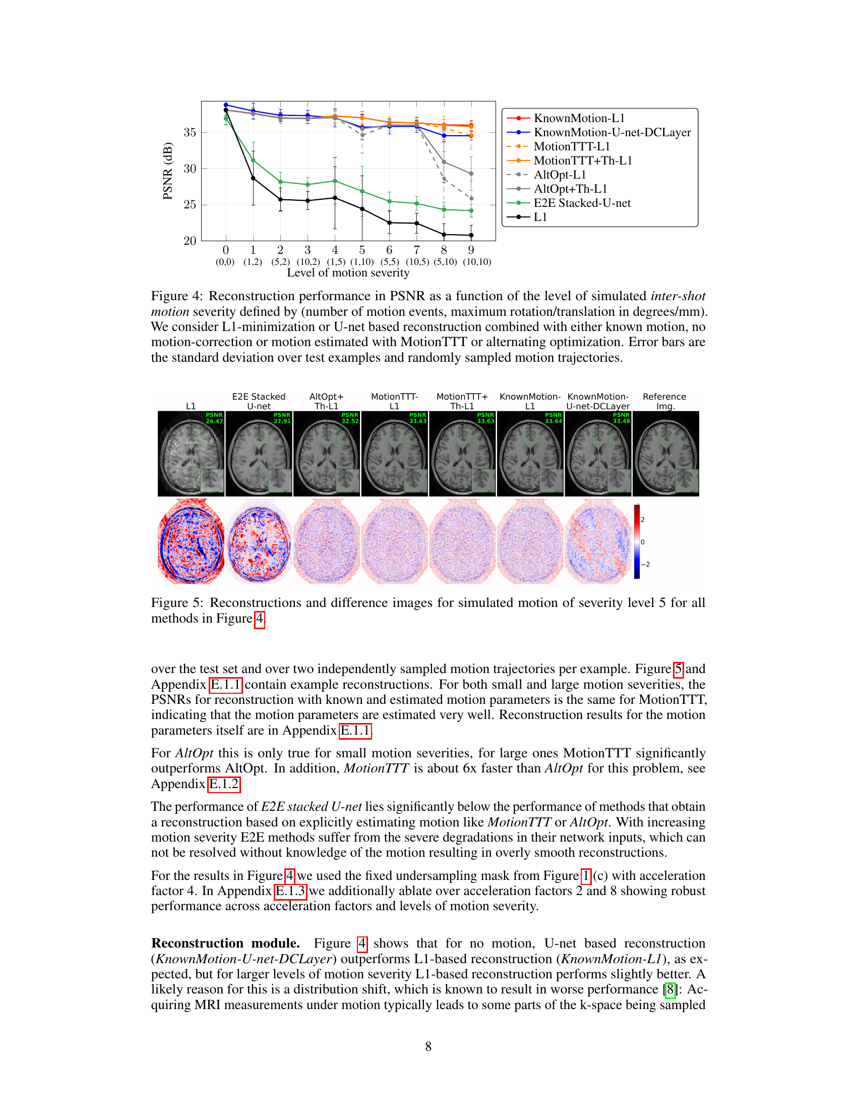
This figure shows the Peak Signal-to-Noise Ratio (PSNR) performance of different motion correction methods across various levels of simulated inter-shot motion. The x-axis represents the motion severity, defined by the number of motion events and the maximum rotation/translation during motion. The y-axis represents the PSNR values. Different methods are compared: L1 minimization with known motion parameters, U-net reconstruction with known motion, MotionTTT with L1 reconstruction, MotionTTT with L1 reconstruction and thresholding, AltOpt with L1 reconstruction, AltOpt with L1 reconstruction and thresholding, and the end-to-end stacked U-net. The error bars represent the standard deviation across different test examples and randomly generated motion trajectories. It demonstrates MotionTTT’s accuracy and speed in estimating motion parameters, even under conditions of significant motion.

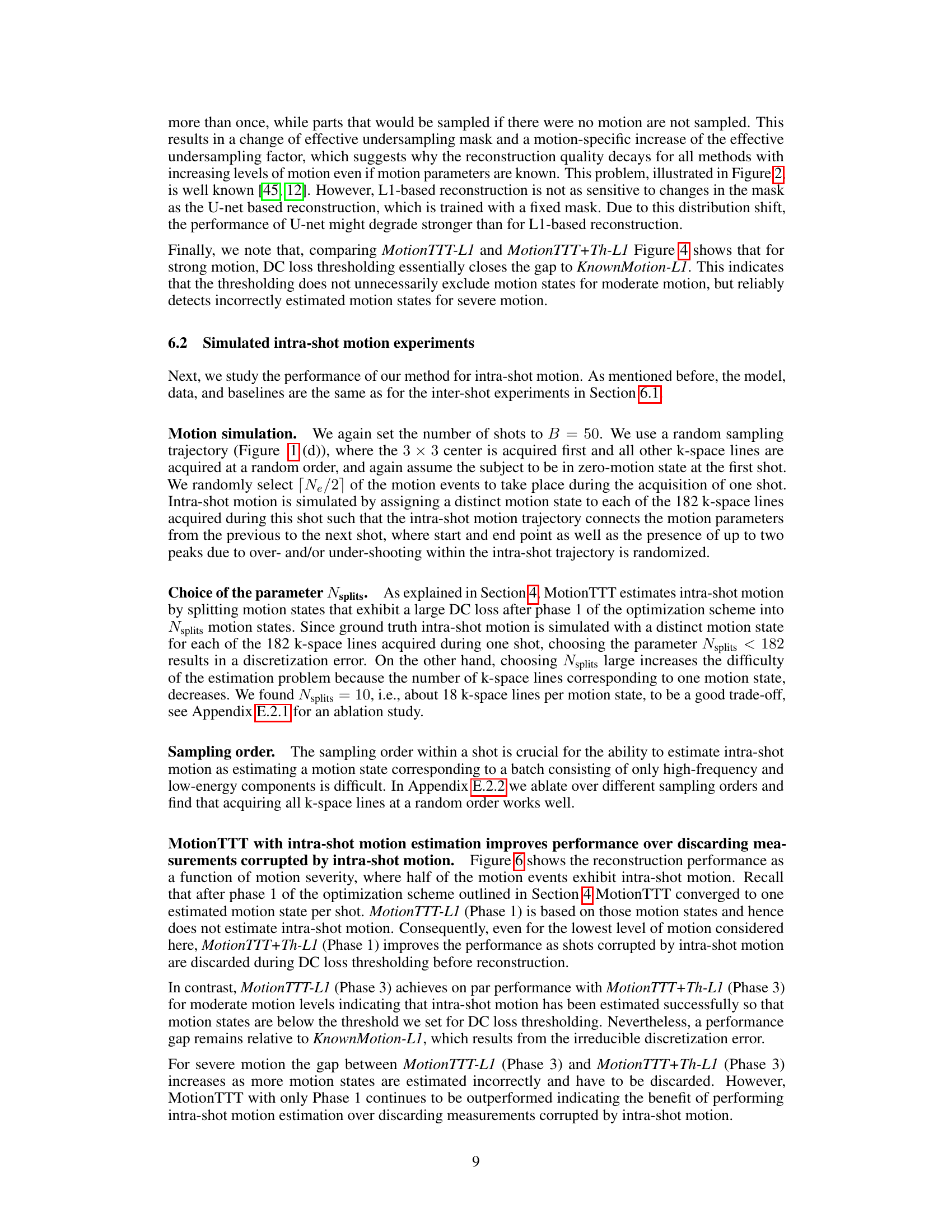
This figure shows a visual comparison of the reconstruction results obtained using different methods for simulated motion with a severity level of 5. It includes the reference image, the reconstructions from L1 minimization, the E2E stacked U-Net, alternating optimization with and without thresholding, and MotionTTT with and without thresholding. Difference images highlight the discrepancies between the reconstructions and the reference image.

This figure shows the PSNR (Peak Signal-to-Noise Ratio) values for different motion correction methods across varying levels of simulated inter-shot motion severity. The x-axis represents the severity level, defined by the number of motion events and the maximum translation or rotation magnitude. The y-axis shows the PSNR. Multiple methods are compared, including using known motion parameters (oracle) for comparison, and methods that estimate motion parameters (MotionTTT, alternating optimization) or no motion correction. The error bars represent the standard deviation across multiple test examples and randomly generated motion trajectories. The results demonstrate the effectiveness of MotionTTT in estimating motion parameters and achieving accurate reconstruction.

This figure compares the visual quality of image reconstructions produced by different methods (L1, E2E Stacked U-Net, AltOpt+Th-L1, MotionTTT-L1, MotionTTT+Th-L1, KnownMotion-L1, KnownMotion-U-net-DCLayer) at different motion severities (levels 1 and 9). The top half shows the results for low severity motion, where the differences between the methods are less pronounced. The bottom half shows the results for high severity motion (level 9), revealing more significant differences in reconstruction quality, particularly highlighting the performance of MotionTTT and KnownMotion methods.
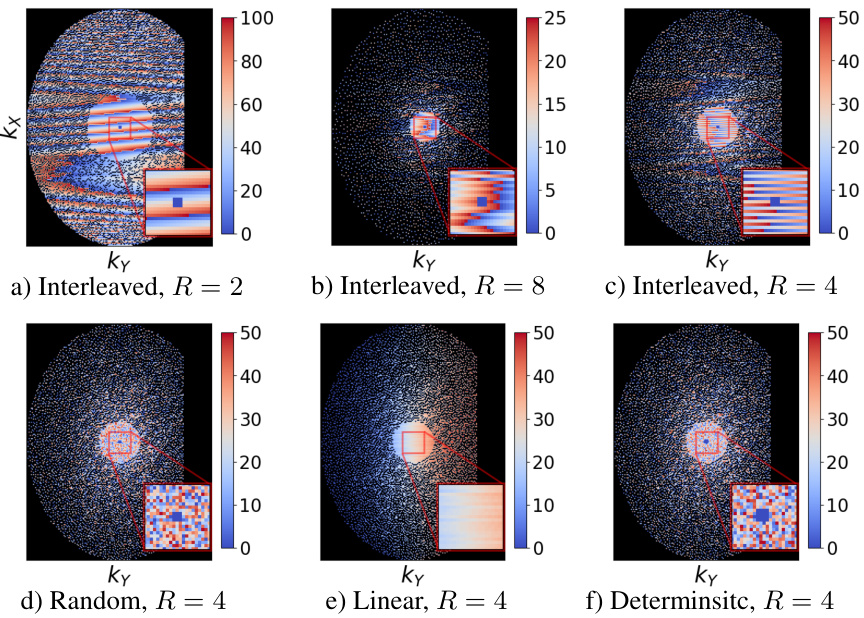
This figure shows six different undersampling masks used in ablation studies to test MotionTTT’s robustness to different sampling strategies. Each mask represents a different acceleration factor (R=2, 4, 8) and sampling trajectory (interleaved, random, linear, deterministic). The color coding helps visualize which k-space lines are sampled within each shot.

This figure shows the performance of different motion correction methods on MRI images with simulated inter-shot motion. The x-axis represents the severity of motion, combining the number of motion events and the maximum rotation/translation magnitude. The y-axis represents the Peak Signal-to-Noise Ratio (PSNR), a measure of image quality. Multiple methods are compared: using known ground truth motion parameters, no motion correction, and motion estimation with MotionTTT or alternating optimization. The results are averaged over multiple examples, and error bars show the standard deviation, indicating the variability in performance.
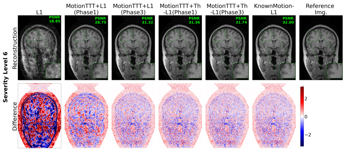
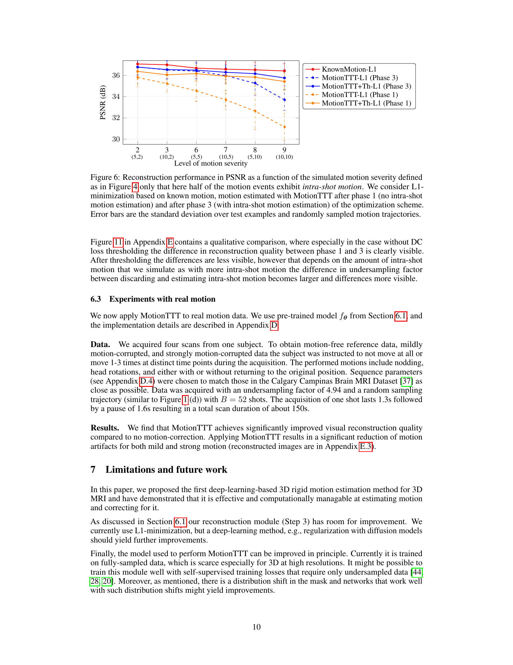
This figure displays a qualitative comparison of reconstruction results using different methods for simulated intra-shot motion with a severity level of 6. It includes the reference image, L1 reconstruction (without motion correction), MotionTTT-L1 (Phase 1, without intra-shot motion estimation), MotionTTT-L1 (Phase 3, with intra-shot motion estimation), MotionTTT+Th-L1 (Phase 1, with DC loss thresholding), MotionTTT+Th-L1 (Phase 3, with DC loss thresholding), and KnownMotion-L1 (reconstruction with known motion parameters). Difference images highlight the discrepancies between the reconstructed images and the reference image, showing how well each method handles the intra-shot motion artifacts. The color scale in the difference images helps to visualize the magnitude and direction of the errors.

This figure shows the visual comparison of MRI reconstructions with real motion data. Three orthogonal planes (axial, sagittal, and coronal) are shown. The columns represent different levels of motion corruption (No motion, Mild Motion 1-3, Strong Motion), and rows represent reconstruction methods (No motion, L1, MotionTTT+Th-L1). The red boxes highlight regions of interest where the improvements by MotionTTT+Th-L1 are particularly apparent. The results show significant improvement in image quality when using MotionTTT+Th-L1, especially with stronger motion artifacts.
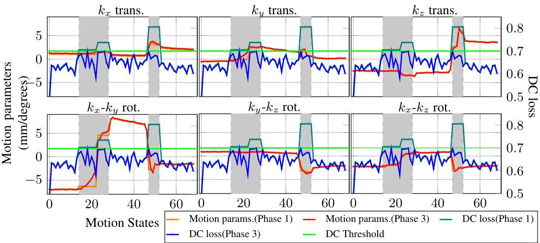
This figure shows the estimated motion parameters (translations and rotations in three dimensions) and the data consistency (DC) loss for each motion state. The data is from a real MRI scan with strong motion. The plot compares the motion parameters estimated in phase 1 (initial estimation) and phase 3 (final estimation) of the MotionTTT algorithm. The gray shaded areas represent intra-shot motion states, meaning that motion occurred within a single shot acquisition, while the white areas represent motion that happened between different shots. The green line indicates the DC loss threshold. Motion states with a DC loss above the threshold are discarded.
More on tables

This table shows the PSNR (Peak Signal-to-Noise Ratio) values and the number of discarded k-space lines for different sampling orders (random, deterministic, interleaved, linear) in the context of MotionTTT+Th-L1 for intra-shot motion correction. It demonstrates the effect of different sampling strategies on reconstruction quality and efficiency by showing the trade-off between PSNR and the number of discarded lines. The higher the PSNR, the better the reconstruction quality; a lower number of discarded lines suggests a more efficient use of acquired data. The results indicate the random and deterministic orders have similar performance.

This table lists the parameters of the 3D T1-weighted Ultrafast Gradient-Echo (TFE) MRI sequence used to acquire the real motion-corrupted data in the experiments described in Section 6.3 of the paper. The parameters include sequence type, flip angle, repetition time (TR), echo time (TE), TFE prepulse and delay, minimum inversion time delay, TFE factor, the number of shots, the duration of each shot and acquisition, the shot interval, sampling type (Cartesian), under-sampling factor, half-scan factors in the Y and Z directions, the number of auto-calibration lines, profile order (random), field of view (FOV), acquisition matrix, fold-over direction, fat shift direction, and water-fat shift. These parameters provide a detailed specification of the MRI acquisition process used in the study.

This table presents the results of the MotionTTT+Th-L1 method under different sampling orders (random, deterministic, interleaved, and linear) for intra-shot motion correction. It shows the average PSNR (Peak Signal-to-Noise Ratio) achieved across four validation examples and five motion trajectories for each sampling order. Additionally, it shows the average number of k-space lines that were discarded due to the DC loss threshold. This data allows for comparing the effectiveness of different sampling strategies under the conditions of the experiment.

This table presents the performance of the MotionTTT+Th-L1 method for intra-shot motion correction using four different sampling orders (random, deterministic, interleaved, and linear). The performance is measured in Peak Signal-to-Noise Ratio (PSNR), and the number of discarded k-space lines (due to a data consistency loss threshold) is also reported for each sampling order. This data helps to analyze the impact of sampling order on the method’s accuracy and efficiency.

This table presents the results of the MotionTTT+Th-L1 method for intra-shot motion correction using four different k-space sampling orders: random, deterministic, interleaved, and linear. The performance is measured by PSNR (Peak Signal-to-Noise Ratio) and the number of k-space lines discarded due to a data consistency (DC) loss threshold. This shows how the choice of sampling order impacts the reconstruction quality and computational efficiency of the method.
Full paper#
