↗ OpenReview ↗ NeurIPS Homepage ↗ Chat
TL;DR#
Current Transformer-based time series forecasting models heavily rely on a ‘patching’ technique for optimal performance. However, this reliance limits their application to tasks with sufficiently long time series. This paper identifies this over-reliance as a key problem, hindering the models’ broader applicability.
To tackle this, the authors introduce DeformableTST. This innovative model uses a new mechanism called ‘deformable attention’ that can effectively identify and focus on important time points within a time series without needing patching. Experimental results demonstrate that DeformableTST consistently achieves state-of-the-art performance, especially in cases where patching is unsuitable, thus significantly enhancing the applicability of Transformer-based forecasting models.
Key Takeaways#
Why does it matter?#
This paper is crucial for time series forecasting researchers as it addresses the over-reliance on patching in Transformer-based models, a significant limitation in current approaches. It proposes DeformableTST, a novel model that achieves state-of-the-art performance across various tasks, particularly those unsuitable for patching. This opens new avenues for improving model applicability and broadening the field’s scope.
Visual Insights#

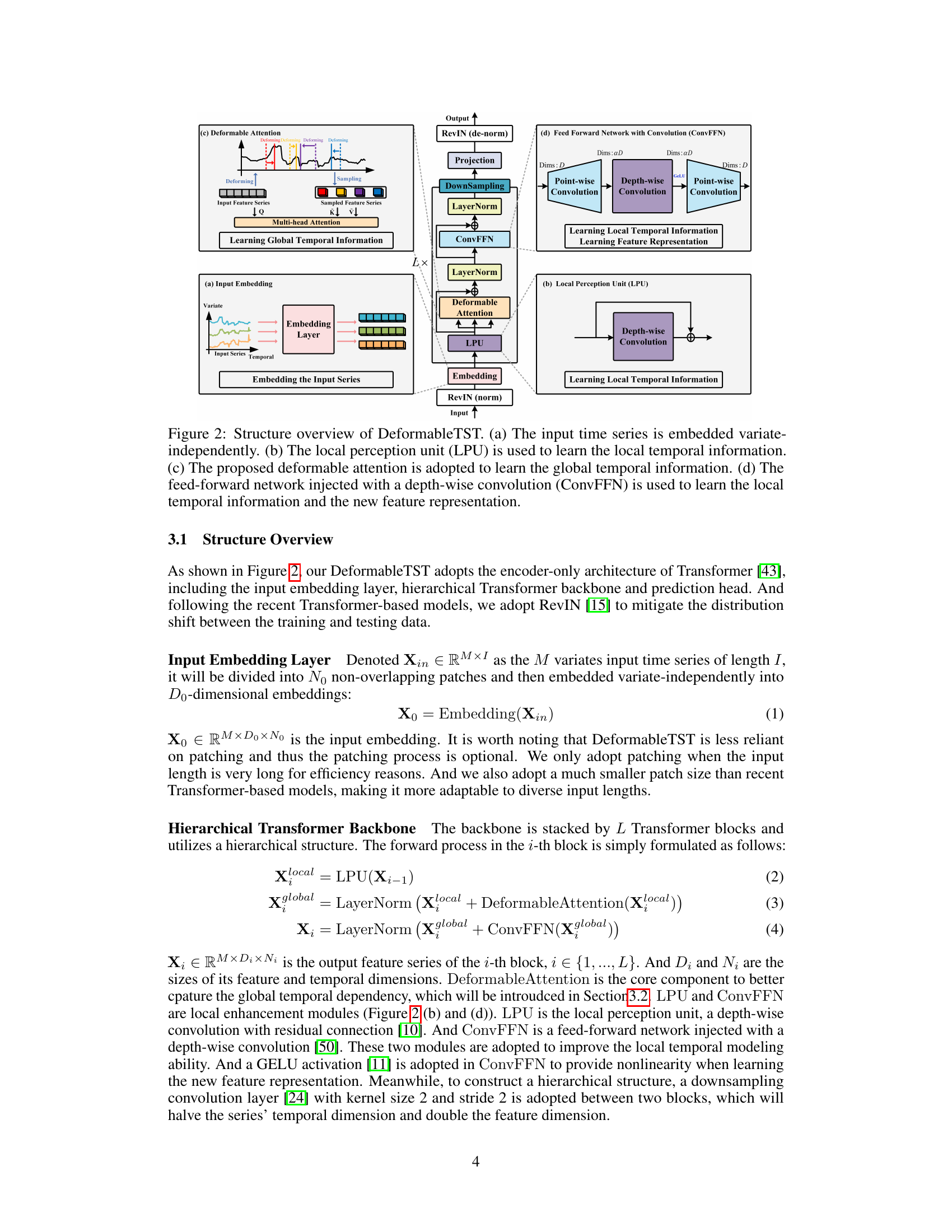
This figure presents a detailed architecture of the proposed DeformableTST model for time series forecasting. It’s broken down into four key components: (a) Input Embedding Layer: The input time series is embedded independently for each variate. (b) Local Perception Unit (LPU): This module processes the embedded input, focusing on learning local temporal relationships using a depth-wise convolution and residual connection. (c) Deformable Attention: This is a crucial component of the model that captures long-range temporal dependencies using a sparse attention mechanism which focuses on important time points to learn non-trivial temporal representations. (d) Feed-Forward Network with Convolution (ConvFFN): This module further refines the feature representation learned from the deformable attention, incorporating both local and global temporal information through a depth-wise convolution and GELU activation. The hierarchical structure is also highlighted, showing how the LPU and deformable attention work together within each Transformer block.

This table presents the results of long-term multivariate time series forecasting experiments using various models. The performance metric used is the Mean Squared Error (MSE) and Mean Absolute Error (MAE). The table compares the performance of the proposed DeformableTST model with several state-of-the-art baselines across different input lengths (I) and prediction lengths (T). Lower MSE and MAE values indicate better performance. The average results across multiple input and prediction lengths are displayed, with references to additional tables for more detailed findings.
In-depth insights#
Patching Dependence#
The concept of “Patching Dependence” highlights a critical limitation of recent Transformer-based time series forecasting models. These models, while achieving impressive results, demonstrate an over-reliance on the “patching” technique—dividing the input time series into smaller segments. This dependence limits their applicability to time series with short lengths or specific structures unsuitable for partitioning. A thoughtful analysis reveals that this reliance stems from the core attention mechanism within Transformers struggling to effectively focus on crucial time points without external guidance from patching. The patching acts as a filter, guiding the model towards relevant temporal information, thus compensating for the attention’s inherent inability to discern importance independently. Therefore, moving beyond patching dependence requires innovative attention mechanisms capable of effectively identifying and prioritizing significant temporal points in a data-driven manner. This may involve exploring sparse attention strategies or other techniques that enhance the capacity of the model to discern meaningful patterns directly from the input data, thereby overcoming the limitation imposed by the need for pre-processing with patching.
Deformable Attention#
The proposed deformable attention mechanism is a data-driven sparse attention method designed to address the over-reliance on patching in transformer-based time series forecasting models. It achieves this by directly learning to focus on important temporal points without the need for explicit patching, a technique previously crucial for the success of such models. This is accomplished through a learnable offset network that samples a subset of key time points from the input sequence, dynamically adapting to the unique characteristics of each time series. By focusing on these selected points, deformable attention efficiently models temporal dependencies and avoids the computational burden and limitations associated with large-scale patching. The resulting model, DeformableTST, exhibits improved performance on a range of time series forecasting tasks, particularly those not suitable for traditional patching techniques, demonstrating the effectiveness of this novel attention approach. The learnable offsets are a key innovation, providing flexibility and adaptability compared to prior-based sparse attention methods, which rely on fixed priors that may not generalize well across diverse datasets. The data-driven nature of deformable attention is crucial to its success in handling varied temporal patterns and complexities inherent in real-world time series data.
Hierarchical Design#
A hierarchical design in deep learning models, particularly for time series forecasting, typically involves a multi-level architecture where each level processes information at a different granularity or scale. Lower levels may focus on extracting local features from the raw time series data, while higher levels integrate those local features to learn global patterns and temporal dependencies. This approach offers several advantages: improved efficiency by processing smaller chunks of data at lower levels, enhanced representation power by capturing both fine-grained and coarse-grained information, and better generalization by learning hierarchical representations that are more robust to noise and variations in the data. However, careful consideration must be given to the design of the inter-level connections and information flow to ensure effective information propagation and prevent information loss or distortion. The optimal depth and width of the hierarchy would depend on the complexity of the time series data and the specific forecasting task. Balancing the trade-off between efficiency and representation power is a key design consideration for such an architecture.
Broader Applicability#
The concept of “Broader Applicability” in the context of a research paper, likely focusing on a novel method or model for time series forecasting, centers on the model’s capacity to effectively handle a wider range of tasks and datasets than existing approaches. Improved performance across various input lengths, data types (univariate or multivariate), and forecasting horizons would be key indicators. The research likely demonstrates this broader applicability through extensive experimentation, showing consistent state-of-the-art or near state-of-the-art results across multiple benchmarks. A critical element is addressing limitations of previous methods, such as over-reliance on specific techniques like patching, which might restrict their applicability. The paper likely argues that the proposed model’s flexibility and adaptability overcome these limitations, thereby expanding the scope of solvable problems within time series forecasting.
Future Research#
Future research directions stemming from this work could explore several promising avenues. Extending DeformableTST to handle high-dimensional multivariate time series is crucial, especially in domains like finance and sensor networks where dealing with numerous interconnected variables is commonplace. This will involve investigating more sophisticated methods for capturing cross-variable dependencies within the deformable attention mechanism. Further research should also focus on improving the efficiency of the model, perhaps through more advanced sparse attention techniques or architectural optimizations designed for memory efficiency on extremely long sequences. Finally, a thorough investigation into the model’s ability to handle various data patterns and noise types is warranted. The robustness of deformable attention should be tested against various levels of noise and irregularities, potentially leading to improved designs. Investigating the transferability and generalizability of DeformableTST across diverse datasets and application domains is also crucial. This will entail applying the model to a wider range of real-world datasets and evaluating its performance against existing benchmarks. Ultimately, these efforts will lead to a more robust and widely applicable forecasting model for various real-world scenarios.
More visual insights#
More on figures
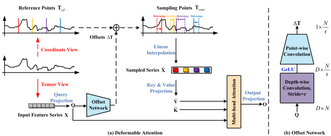
This figure illustrates the deformable attention mechanism. (a) shows the process from both tensor and coordinate views. The input feature series X first samples a few important time points based on learnable offsets. Then these sampled points are fed to key and value projections (K, V), while X is projected to queries Q. Finally, multi-head attention is applied to Q, K, and V to get the output O. (b) shows the structure of the offset network that generates the offsets. It consists of a depthwise convolution followed by a pointwise convolution, using GELU activation and producing offsets ∆T.

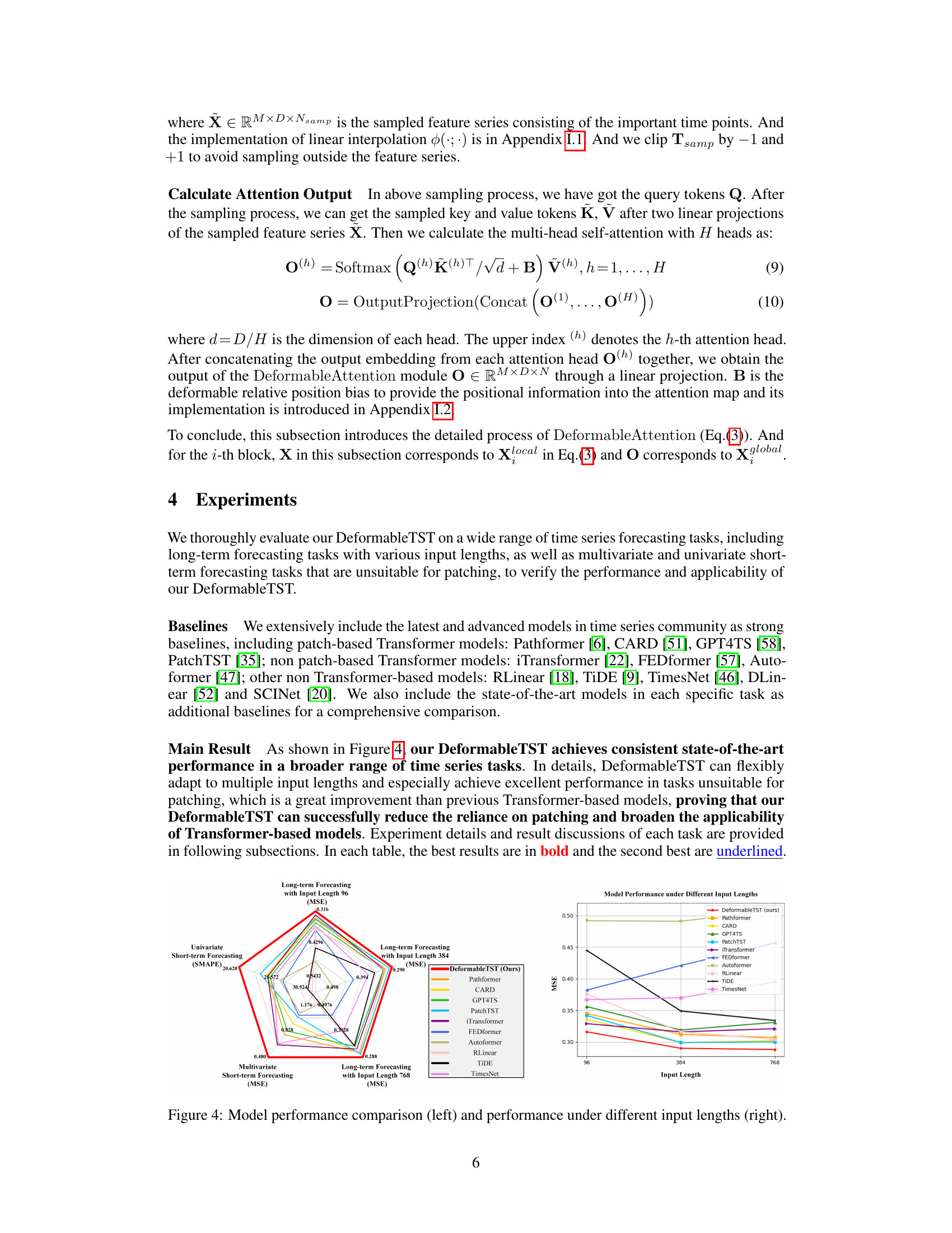
The left part of the figure is a radar chart comparing the performance of DeformableTST against other state-of-the-art models across various time series forecasting tasks: univariate short-term forecasting (SMAPE), multivariate short-term forecasting (MSE), long-term forecasting with input lengths 96, 384, and 768 (MSE). The right part shows a line graph illustrating how the MSE changes for each model with different input lengths. This visualization helps understand the model’s adaptability to various input lengths and task types, especially highlighting DeformableTST’s consistent superior performance.

This ablation study visualizes the effect of each design choice made to improve PatchTST and arrive at DeformableTST. It shows the impact of removing patching, adding a hierarchical structure, incorporating deformable attention, and adding local enhancement modules on both model performance (MSE) and memory usage. The results demonstrate that each addition contributes to improved performance and efficiency.

This figure presents a comparison of the model’s performance against other state-of-the-art models on various time series forecasting tasks. The left panel shows a performance comparison across different datasets, illustrating the model’s consistent superiority. The right panel visualizes performance as a function of input length, demonstrating the model’s adaptability and effectiveness even with shorter sequences, which is a key advantage over models that heavily rely on patching.
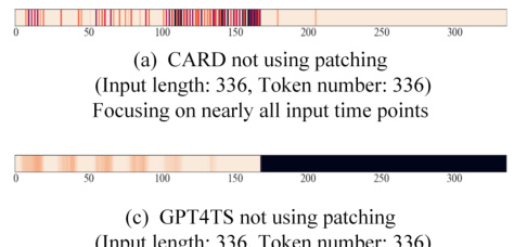
The figure visualizes the effective receptive fields (ERFs) of the PatchTST model with and without patching. The ERF shows which time points the model focuses on when extracting temporal representations. The visualization demonstrates that when using patching (dividing the time series into patches), PatchTST concentrates attention on a smaller set of important time points, achieving better performance. In contrast, without patching, the model’s attention is spread thinly across nearly all time points, resulting in poorer performance. This highlights PatchTST’s over-reliance on the patching technique. The same phenomenon is also observed in other advanced patch-based Transformer models.

This figure visualizes the effective receptive fields (ERFs) of the PatchTST model with and without patching. The ERF shows which parts of the time series the model focuses on when learning temporal representations. The visualization reveals that when using patching, the model focuses on a smaller subset of key time points, while without patching, the model attends to almost all time points equally. This demonstrates PatchTST’s strong reliance on patching to achieve optimal performance. The appendix further supports this finding by showing that multiple advanced patch-based transformer models exhibit the same behavior.

The figure visualizes the effective receptive fields (ERFs) of the PatchTST model with and without patching. The ERF shows which time points in the input time series are focused on by the model during temporal representation learning. The results demonstrate that PatchTST heavily relies on patching to effectively focus on important time points, highlighting a potential over-reliance on this technique in current Transformer-based forecasting models. The phenomenon is also observed in other advanced patch-based Transformer models.

This figure visualizes the effective receptive fields (ERFs) of the DeformableTST model. The ERF shows which parts of the input time series are focused by the model when extracting temporal representations. Brighter areas indicate that those time points are more important for the model to focus on when learning temporal representations. This visualization helps to understand how the DeformableTST model focuses on important time points to learn non-trivial temporal representation, which is crucial for accurate time series forecasting, especially when dealing with tasks where patching is not suitable.

This ablation study shows the effect of each component in DeformableTST by gradually adding components to PatchTST. It demonstrates that removing patching initially worsens performance and memory usage. However, adding hierarchical structure, deformable attention, and local enhancement improves performance and reduces memory usage, ultimately leading to DeformableTST’s superior performance and efficiency compared to the original PatchTST.
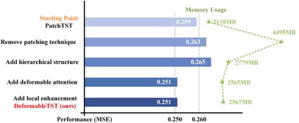
This ablation study shows the impact of each component of DeformableTST on the model’s performance and memory usage. Starting with PatchTST, each component is added sequentially, showing the improvements in MSE and memory usage. The results demonstrate that removing patching initially hurts performance, but adding hierarchical structure, deformable attention, and local enhancement improves it again, resulting in a more efficient and better-performing model than PatchTST.

This ablation study demonstrates the impact of each design choice in DeformableTST on its performance and memory usage. Starting from PatchTST, modifications are made sequentially: removing patching, adding a hierarchical structure, incorporating deformable attention, and finally adding local enhancement. The results show that while removing patching initially hurts performance and significantly increases memory usage, the subsequent design choices mitigate these issues and lead to a superior model (DeformableTST) with better performance and lower memory.

This figure illustrates the deformable attention mechanism proposed in the paper. Panel (a) shows the process of deformable attention from both tensor and coordinate perspectives, highlighting the sampling of important time points from the input feature series based on learnable offsets. These points are used to compute the attention mechanism. Panel (b) details the structure of the offset network, which generates these learnable offsets. The network’s input is the query tokens, and it uses depth-wise and point-wise convolutions with a GeLU activation to output the offsets.
The figure on the left shows the overall performance of DeformableTST against other models on various time series forecasting tasks, indicating its state-of-the-art performance. The figure on the right specifically analyzes performance across different input lengths, highlighting DeformableTST’s consistent high performance and adaptability to diverse input lengths compared to other models, which tend to struggle with shorter sequences.

This figure presents a comparison of the model’s performance against other state-of-the-art models. The left panel displays a comparison of the overall performance across various time series forecasting tasks, while the right panel shows a performance comparison under different input lengths. The results demonstrate that DeformableTST consistently outperforms other methods, especially for tasks with shorter input lengths, unsuitable for traditional patching techniques.

This figure shows a comparison of the model’s performance with other state-of-the-art models on several time series forecasting tasks. The left panel presents a comparison of the overall performance (measured by MSE for long-term forecasting tasks and SMAPE for short-term forecasting tasks) across different datasets. The right panel shows how the model’s performance changes with varying input sequence lengths, highlighting the model’s ability to adapt to various input lengths and perform consistently well.
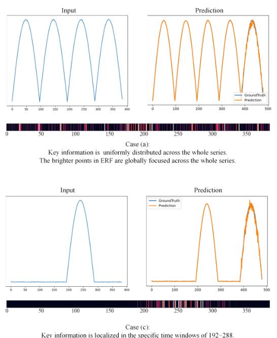
The figure visualizes the effective receptive field (ERF) of the PatchTST model, highlighting its reliance on patching to focus on important time points during temporal representation extraction. It contrasts the ERF when using patching (focusing on key points) versus not using patching (focusing on almost all points equally), illustrating how patching guides the model toward more meaningful temporal representations. The results demonstrate that without patching, the model has not effectively learned the importance of individual time points, leading to inferior forecasting performance. This over-reliance on patching is also seen in other advanced patch-based Transformer models.

This figure shows a comparison of the model’s performance against other state-of-the-art models on various time series forecasting tasks. The left panel presents a comparison of overall performance metrics (e.g., MSE, SMAPE) across different datasets, while the right panel analyzes how the model’s performance changes with varying input lengths. This illustrates the model’s adaptability to a wide range of input sizes and its ability to maintain strong performance even with shorter input sequences, which is a key advantage highlighted in the paper.

This figure presents a comprehensive comparison of DeformableTST’s performance against various state-of-the-art models across different time series forecasting tasks. The left panel shows the model’s overall performance across multiple tasks, while the right panel displays performance under varying input lengths. This demonstrates DeformableTST’s adaptability and consistent performance across a broader range of forecasting scenarios compared to existing methods.
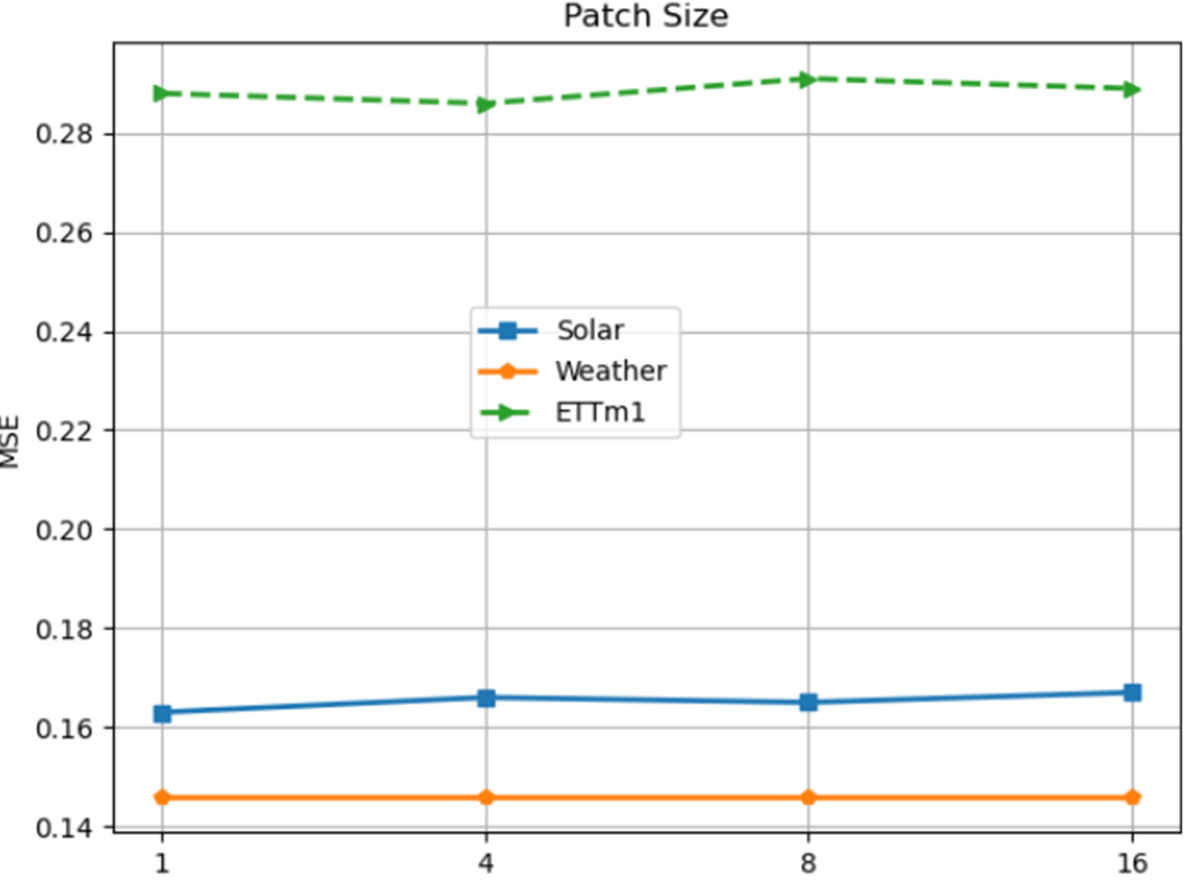
The figure shows the sensitivity analysis of the DeformableTST model’s performance to different hyperparameters. For the patch size, experiments are conducted with input length 384 and prediction length 96, using PatchTST as a baseline for comparison. For other hyperparameters (model dimension, FFN expansion, number of blocks, number of important time points, and learning rate), experiments are conducted with input length 96 and prediction length 96. The results visualize the robustness of the model to the hyperparameter choices and demonstrate that its performance is relatively stable across various settings.
More on tables

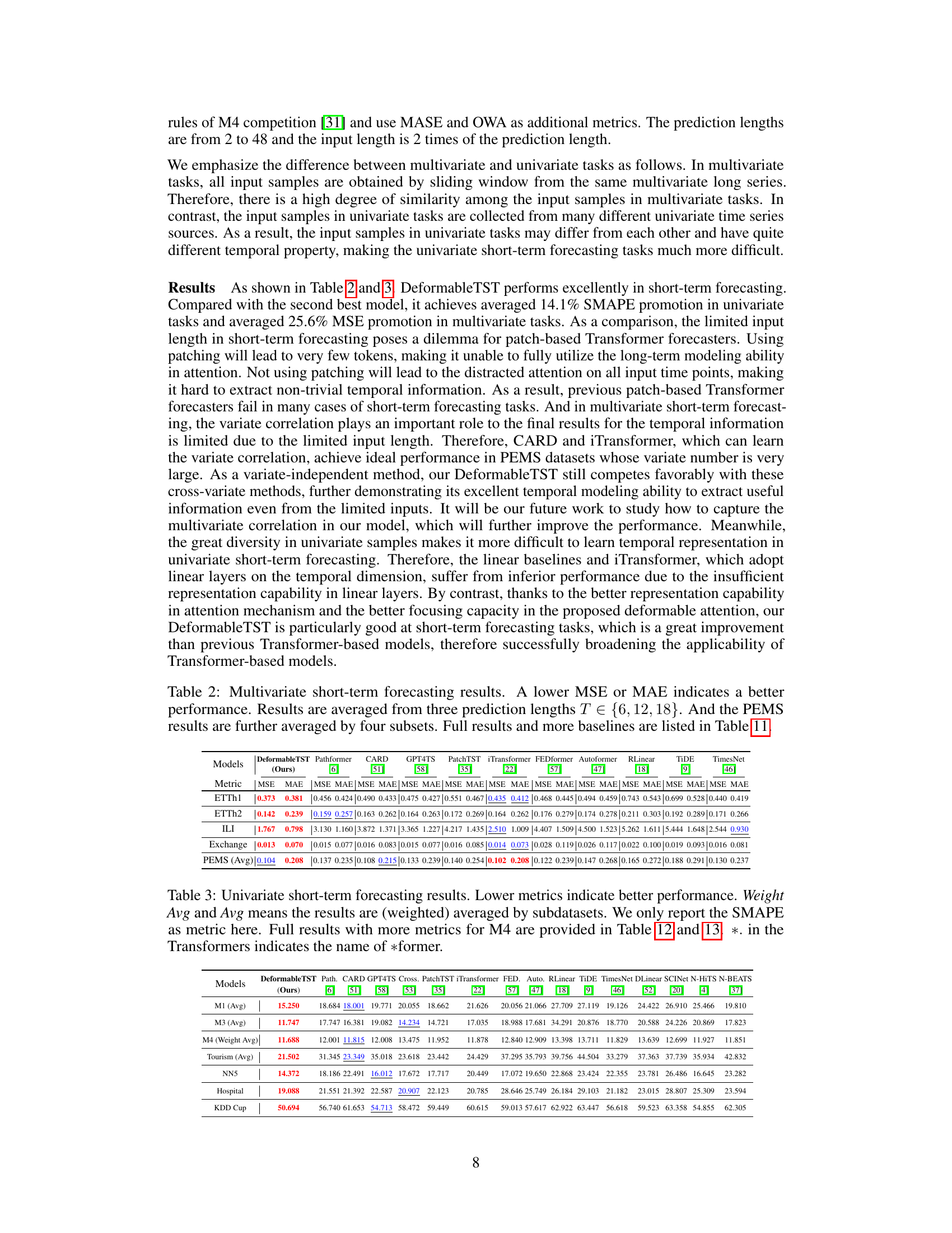
This table presents the results of multivariate short-term forecasting experiments. It compares the performance of DeformableTST against several other state-of-the-art models across multiple datasets. The input length is twice the prediction length. The average performance across three different prediction lengths (6, 12, and 18) is reported, offering a comprehensive comparison of the models’ effectiveness in this type of forecasting task.

This table presents a detailed comparison of various models’ performance on multivariate short-term forecasting tasks. It shows the mean squared error (MSE) and mean absolute error (MAE) for each model across three prediction lengths (6, 12, 18). The input sequence length is always twice the prediction length. The ‘Avg’ column provides the average performance across these three prediction lengths. The table allows for a comprehensive assessment of different models’ capabilities in handling multivariate short-term forecasting problems.

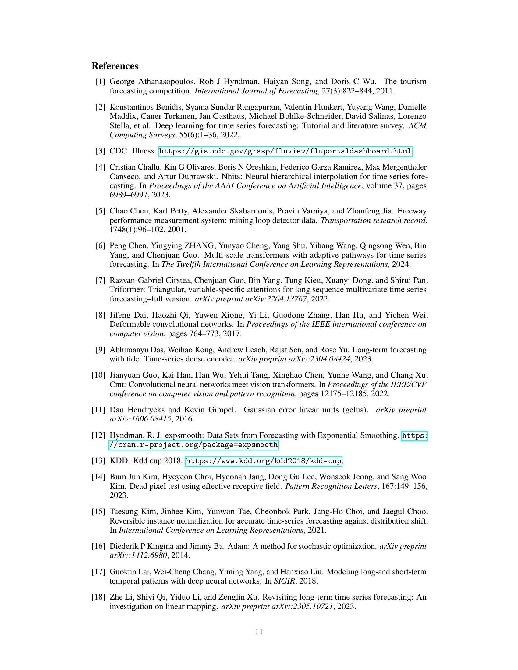
This table compares the performance of the proposed deformable attention mechanism against other prior-based sparse attention mechanisms commonly used in time series forecasting. The comparison is conducted within the context of long-term forecasting tasks using an input sequence length of 96. The table presents the average Mean Squared Error (MSE) and Mean Absolute Error (MAE) across four different prediction lengths. The results highlight the superior performance of the deformable attention, showcasing its effectiveness in capturing temporal dependencies.

This table provides detailed information about the multivariate datasets used in the paper for both long-term and short-term forecasting experiments. For each dataset, it lists the task (long-term or short-term forecasting), the dataset name, the number of variates, the prediction lengths used, the dataset sizes (train, validation, test splits), the data frequency (hourly, 15min, 5min, daily, weekly), and the type of information contained within the dataset (electricity, weather, transportation, illness, economy). This information is crucial for understanding the experimental setup and the scope of the results presented.

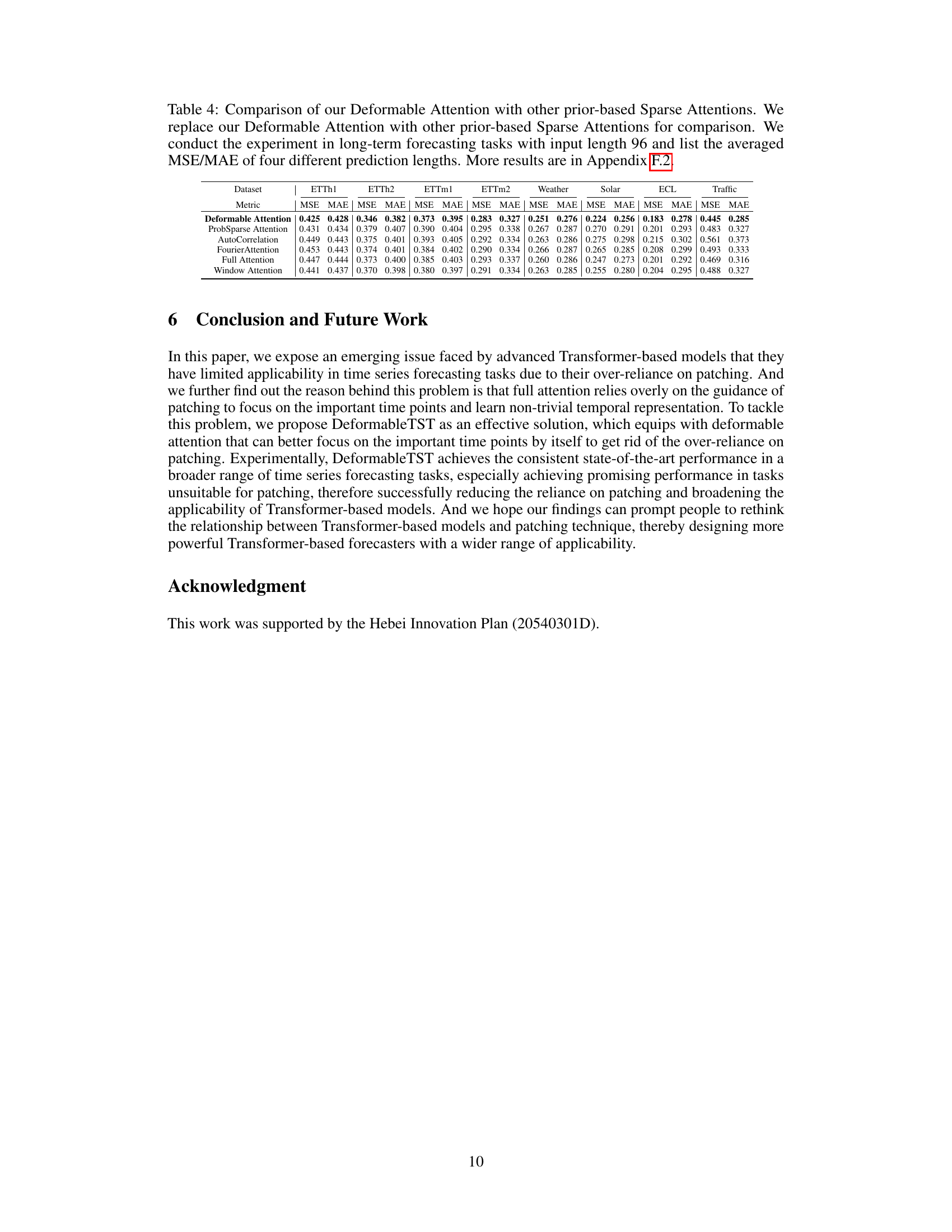
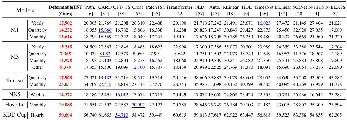
This table presents the details of the univariate short-term forecasting datasets used in the paper. It includes the dataset name, the number of samples in the training, validation, and test sets, the number of variables, and the prediction length for each dataset. The datasets cover various frequencies (yearly, quarterly, monthly, weekly, daily, and hourly) and represent various application domains, including macroeconomics, microeconomics, industry, finance, and tourism.

This table presents the standard deviation of the DeformableTST’s performance across five independent runs with different random seeds. The results are presented for multiple datasets (ETTh1, ETTh2, ETTm1, ETTm2, Weather, Solar-Energy, ECL, Traffic) and prediction horizons (96, 192, 336, 720). It shows the stability of the model’s performance across multiple runs.

This table presents the results of multivariate long-term time series forecasting experiments. The Mean Squared Error (MSE) and Mean Absolute Error (MAE) are reported as metrics. Results are averaged across three different input lengths (96, 384, and 768 time steps) and four prediction lengths (96, 192, 336, and 720 time steps) to demonstrate the model’s adaptability and consistency. The table compares the performance of DeformableTST against several state-of-the-art baselines on multiple datasets. More detailed results and comparisons with additional baselines are available in Tables 8, 9, and 10.

This table presents the complete results of the long-term forecasting experiments with an input length of 96 time steps. It compares the performance of DeformableTST against several other state-of-the-art models across four different prediction lengths (96, 192, 336, and 720). The ‘Avg’ row shows the average performance across all prediction lengths. The metrics used are MSE (Mean Squared Error) and MAE (Mean Absolute Error). The table allows for a comprehensive comparison of the models under various prediction horizons.

This table presents a detailed comparison of the model’s performance on multivariate short-term forecasting tasks against several other state-of-the-art models. It shows Mean Squared Error (MSE) and Mean Absolute Error (MAE) for different prediction lengths (6, 12, and 18), averaged across multiple datasets, offering a comprehensive evaluation of the DeformableTST’s performance relative to its competitors.

This table presents a comprehensive comparison of various models’ performance on multivariate short-term forecasting tasks. It shows the Mean Squared Error (MSE) and Mean Absolute Error (MAE) for different prediction lengths (6, 12, and 18 time steps), averaged across the three lengths. The input sequence length for each prediction length was twice as long. Multiple datasets are included in the comparison.

This table presents a comprehensive comparison of various time series forecasting models on multivariate short-term forecasting tasks. It shows the Mean Squared Error (MSE) and Mean Absolute Error (MAE) for different models across three prediction lengths (6, 12, and 18 time steps). The input sequence length is twice the prediction length for all models. The average performance across all three prediction lengths is also provided.
This table presents a detailed comparison of the DeformableTST model with various other competitive models on eight multivariate short-term time series forecasting datasets. The models are evaluated on three different prediction lengths (6, 12, and 18 time steps), with the input length always double the prediction length. The table shows Mean Squared Error (MSE) and Mean Absolute Error (MAE) for each model on each dataset and prediction length, along with an average across all prediction lengths. This allows for a comprehensive assessment of model performance in this type of task.

This table compares the performance of DeformableTST and Sageformer on eight long-term forecasting datasets. The metrics used are Mean Squared Error (MSE) and Mean Absolute Error (MAE). The results are averaged across three different input lengths (96, 384, and 768) and four prediction lengths (96, 192, 336, and 720). DeformableTST consistently outperforms Sageformer.

This table presents a comprehensive comparison of the DeformableTST model’s performance against the Sageformer model in long-term time series forecasting. It shows the Mean Squared Error (MSE) and Mean Absolute Error (MAE) for both models across four different prediction lengths (96, 192, 336, and 720) and eight different datasets (ETTh1, ETTh2, ETTm1, ETTm2, Weather, Solar, ECL, and Traffic). The results are averaged across three different input lengths (96, 384, and 768) to demonstrate the models’ performance robustness across varying data lengths.

This table presents a comparison of various time series forecasting models on the Stock Market dataset for short-term predictions. It shows the Mean Squared Error (MSE) and Mean Absolute Error (MAE) achieved by different models across three prediction lengths (6, 12, and 18 time steps), with the input length being twice the prediction length. The table highlights the superior performance of DeformableTST, showcasing its adaptability and accuracy compared to other state-of-the-art methods.
Full paper#
