↗ OpenReview ↗ NeurIPS Homepage ↗ Chat
TL;DR#
Current score-based generative models, while successful, suffer from issues like slow convergence, mode collapse, and lack of diversity, often stemming from using Brownian motion (BM) with independent increments. The limitations of BM, particularly its light-tailed nature and Markovian property, restrict the models’ ability to capture the complexity and richness of real-world data. There have been attempts to address this by incorporating different noise types, but these often come with computational challenges or theoretical intractability.
This paper proposes a solution by using fractional Brownian motion (fBM), which has correlated increments and a Hurst index that controls its roughness and long-range dependence. The authors overcome the computational challenges of fBM using a Markov approximation and derive a reverse-time model, leading to Generative Fractional Diffusion Models (GFDM). They introduce augmented score matching for efficient training and demonstrate that GFDM achieves improved pixel-wise diversity and image quality on image datasets, showcasing its potential as a promising alternative to traditional diffusion models.
Key Takeaways#
Why does it matter?#
This paper is significant because it introduces a novel generative model that uses fractional Brownian motion, improving the quality and diversity of generated images. It addresses limitations of existing diffusion models and offers a new approach to generative modeling, opening avenues for further research in this area. This is particularly relevant given the recent surge in interest and advancements in score-based generative models.
Visual Insights#

This figure illustrates the data dimension transitions to a known prior distribution using a forward process approximating fractional diffusion. The Hurst index (H) controls the roughness of the process, interpolating between Brownian motion (BM) and the probability flow ODE integration. Correlated processes, driven by the same BM, form the driving noise. Importantly, the score function for these processes has a closed-form solution, aiding in learning the unknown score function.
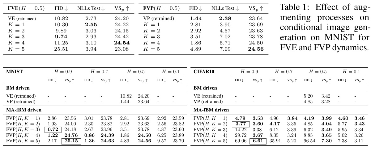
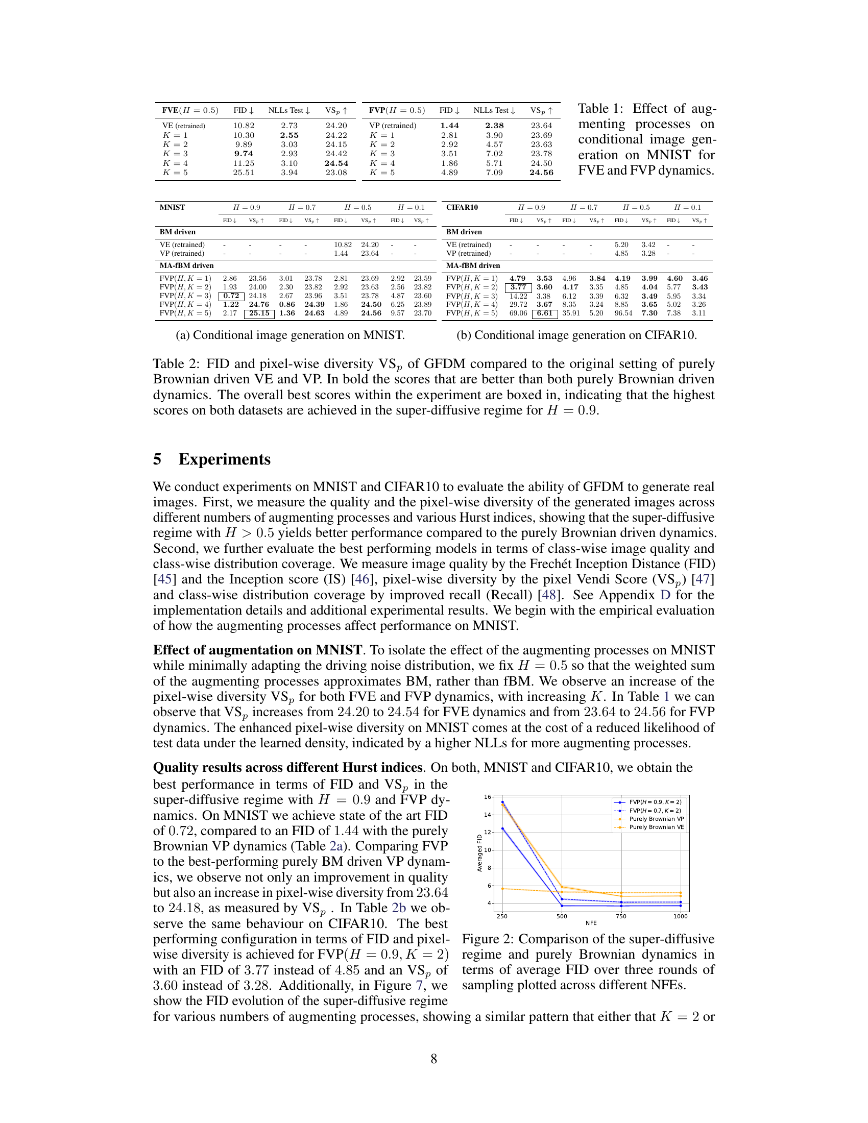
This table shows the impact of increasing the number of augmenting processes (K) on the quality of generated images, specifically focusing on two different dynamics, Fractional Variance Exploding (FVE) and Fractional Variance Preserving (FVP), using the MNIST dataset. Metrics evaluated include FID (Frechét Inception Distance) for image quality, NLLs Test for likelihood, and VSp (Pixel Vendi Score) for pixel diversity. The results show how adding more processes can affect the balance between image quality and diversity at different Hurst indices (H).
In-depth insights#
FracDiff Background#
The heading ‘FracDiff Background’ suggests a section dedicated to the foundational concepts of fractional diffusion and its relevance to the research. It would likely cover the mathematical underpinnings of fractional Brownian motion (fBM), contrasting it with standard Brownian motion. Key differences such as the presence of long-range dependence and self-similarity in fBM, characterized by the Hurst exponent, would be highlighted. The section would also discuss existing applications of fractional diffusion models and address why they are considered advantageous or necessary for the particular research problem, potentially focusing on their ability to capture complex temporal dependencies in data or improved performance in generative models. The background would provide context for the proposed methods, laying the groundwork for understanding the innovations presented in the paper. A thorough review of relevant literature within the field of fractional calculus and its applications within the specific domain of the research would be expected, establishing the significance and novelty of the presented work within this context. Finally, any limitations or challenges associated with applying fractional diffusion models would also be discussed.
GFDM Training#
GFDM training, as described in the paper, presents a novel approach to training score-based generative models using a Markov-approximated fractional Brownian motion (MA-fBM). This method directly addresses limitations of traditional diffusion models by incorporating correlated noise and long-term memory. The core of GFDM training involves learning the score function using an augmented score matching loss. This approach cleverly reduces computational cost by focusing on data-dimensionality instead of the higher dimensionality inherent in the augmented process. The training procedure leverages a continuous reparameterization trick for efficient sampling, further improving the training process’s stability and speed. The Hurst index (H), a crucial parameter controlling the roughness of the MA-fBM, provides additional flexibility and control over the generation process, allowing for fine-tuning of generated data diversity and fidelity. The results demonstrate that the GFDM method achieves enhanced performance compared to traditional models, specifically showing increased pixel-wise diversity and improved image quality. Overall, the GFDM training strategy showcases a sophisticated and effective solution for generative modeling that harnesses the strengths of fractional diffusion processes while mitigating their inherent computational challenges.
Rough Path Effects#
The concept of ‘Rough Path Effects’ in the context of generative models using fractional Brownian motion (fBM) is intriguing. fBM’s non-Markovian nature, characterized by its Hurst exponent H, introduces dependencies between increments, unlike the independent increments of Brownian motion. When H<0.5, paths are considered ‘rough’, leading to potentially significant effects on the model’s dynamics and learning. Rough paths might enhance the model’s ability to capture complex, long-range dependencies in data, allowing for greater expressiveness and potentially mitigating mode collapse. However, the increased roughness also presents challenges for inference and learning, requiring novel techniques such as Markov approximations of fBM. The reverse-time model derivation becomes more complex, impacting the efficiency of sample generation. Careful consideration of the computational cost and stability of numerical methods is crucial when dealing with the increased complexity introduced by rough path effects. Further research into the optimal H value and the trade-off between expressiveness and computational tractability is necessary to fully understand the potential benefits of exploiting rough path effects.
GFDM Limitations#
Generative Fractional Diffusion Models (GFDM), while showing promise, have limitations. Computational cost increases with more augmenting processes, impacting efficiency. The Markov approximation of fBM introduces error, potentially affecting the quality and diversity of generated samples. Generalization to diverse datasets beyond MNIST and CIFAR10 needs further investigation. The optimal Hurst index (H) and number of augmenting processes (K) aren’t universally determined, requiring dataset-specific tuning. Evaluating the effect of these hyperparameters requires substantial computational resources. Finally, the theoretical framework’s complexity might limit broad adoption and further research on the reverse-time model is needed for a deeper understanding.
Future Directions#
Future research could explore applying the GFDM framework to diverse data modalities beyond images, such as time series data or point clouds. Investigating optimal Hurst index values for different data types would be crucial. A theoretical analysis of the limiting behavior of GFDM with infinitely many augmenting processes, and its connection to true fBM reverse-time models, is needed. Developing techniques for switching between two unknown distributions using MA-fBM driven dynamics holds potential for modeling real-world transitions. The practical implications and potential biases of using GFDM in applications like molecular structure generation and drug discovery deserve further study, alongside the development of safeguards against misuse. Addressing the computational cost of higher-dimensional MA-fBM approximations is important for scaling to larger datasets. Lastly, enhancing the qualitative understanding of the relationship between the Hölder exponent, diffusion process roughness, and the quality of generated samples warrants further investigation.
More visual insights#
More on figures

The figure illustrates the forward and reverse processes of the generative fractional diffusion model (GFDM). The left-hand side (LHS) shows how each data dimension transitions to a known prior distribution using a fractional diffusion process, with the Hurst index (H) controlling the roughness of the path. The right-hand side (RHS) shows that this fractional diffusion process is approximated by a combination of correlated Ornstein-Uhlenbeck (OU) processes all driven by the same Brownian motion. The score function for these OU processes is known and guides the learning of the score function for the main diffusion process.
This figure illustrates the forward process in the GFDM model. Each data dimension undergoes a transformation to a known prior distribution via a forward stochastic differential equation (SDE). The Hurst index (H) controls the roughness of this process, interpolating between the smoothness of a Brownian motion (H=0.5) and rougher paths (H<0.5 or H>0.5). The forward process is driven by a fractional Brownian motion (fBM), approximated using a Markov approximation (MA-fBM) which is a linear combination of correlated Ornstein-Uhlenbeck (OU) processes. The score function for these OU processes is known analytically and informs learning of the score function for the main process.

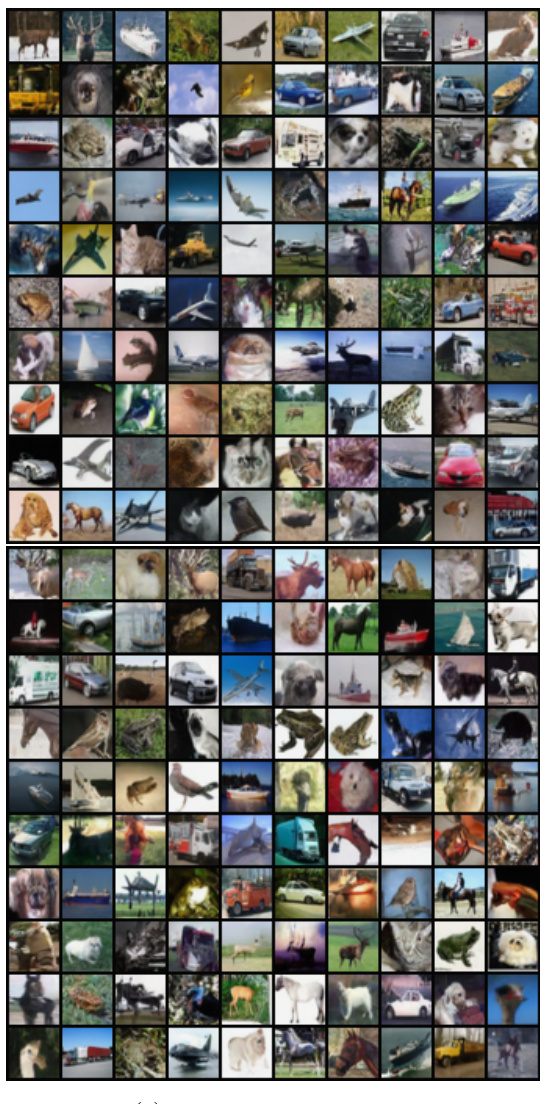
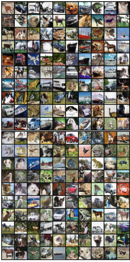
This figure shows a visual comparison of generated CIFAR10 images. The left side displays images generated using purely Brownian driven VP dynamics with the SDE method, resulting in a FID of 4.85 and a pixel-wise diversity of 3.42. The right side shows images generated using the super-diffusive regime of MA-fBM (FVP(H = 0.9, K = 2)) dynamics with the SDE method. This resulted in a FID of 3.77 and higher pixel-wise diversity of 3.60. The figure illustrates the impact of using fractional Brownian motion and the proposed augmented score matching on image quality and diversity.

This figure illustrates the forward process of the GFDM, showing how each data dimension transitions to a known prior distribution. The left-hand side (LHS) depicts a fractional diffusion process approximated by a stochastic differential equation (SDE), controlled by the Hurst index H. The right-hand side (RHS) shows how the driving noise, a fractional Brownian motion (fBM), is approximated by a combination of correlated Ornstein-Uhlenbeck (OU) processes, all driven by the same Brownian motion. The known score function of these OU processes provides guidance for learning the unknown score function of the overall diffusion process.

This figure illustrates the data transition process in the generative fractional diffusion model (GFDM). The left-hand side (LHS) shows a fractional diffusion process where the Hurst index (H) controls the roughness of the path. This process interpolates between the smoothness of a standard Brownian motion (H=0.5) and rougher paths (H<0.5) or smoother paths (H>0.5). The right-hand side (RHS) shows how the driving noise process for the fractional diffusion is a combination of correlated Ornstein-Uhlenbeck (OU) processes, all driven by the same Brownian motion. The score function (used for efficient learning) of these OU processes is already known, and this serves as guidance in learning the score function for the main fractional diffusion process.

This figure illustrates the data dimension transitions in a generative fractional diffusion model. The left-hand side (LHS) shows a fractional diffusion process with a Hurst index H, which controls the roughness of the process. The right-hand side (RHS) depicts the driving noise process as a linear combination of correlated Ornstein-Uhlenbeck (OU) processes, all driven by the same Brownian motion. The score function of these OU processes is known and serves as guidance for the unknown score function of the overall diffusion process.

This figure illustrates the forward process of the GFDM. The left-hand side (LHS) shows how each data dimension transitions to a known prior distribution via a stochastic differential equation (SDE) approximating a fractional diffusion process. The Hurst index H controls the roughness of the process. The right-hand side (RHS) depicts the driving noise process as a linear combination of correlated Ornstein-Uhlenbeck (OU) processes. These OU processes are driven by the same Brownian motion. Notably, the score function of the OU processes is available in closed-form and helps learn the score function for the overall GFDM.

This figure illustrates the data dimension transitions using a forward process which approximates a fractional diffusion process. The left-hand side (LHS) shows how the Hurst index (H) influences the roughness of the process, interpolating between a Brownian driven stochastic differential equation (SDE) and probability flow ordinary differential equations (PF ODEs). The right-hand side (RHS) depicts the driving noise process as a linear combination of correlated processes, all driven by the same Brownian motion. Importantly, the score function for these augmenting processes has a known closed form, providing guidance for determining the unknown score function.
This figure illustrates the transition of data dimensions to a prior distribution using a forward process approximating fractional diffusion. The left side (LHS) shows how the Hurst index (H) controls the roughness of the process, interpolating between Brownian motion (H=0.5) and other fractional Brownian motions. The right side (RHS) details the driving noise as a linear combination of correlated processes, all driven by the same Brownian motion. Importantly, the score function for these augmenting processes has a closed-form solution, guiding the estimation of the unknown score function for the overall process.
The figure illustrates the data dimension transitions to a known prior distribution through a forward process. It shows how the Hurst index H affects the roughness of a Brownian-driven stochastic differential equation (SDE) and the underlying integration in probability flow ordinary differential equations (PF ODEs). The driving noise is a linear combination of correlated processes, all driven by the same Brownian motion. The score function of the augmenting processes (which is known) guides the learning of the unknown score function.
This figure illustrates the transition of data dimensions to a prior distribution using a forward process approximating fractional diffusion. The left-hand side (LHS) shows how the Hurst index (H) controls the roughness of the process, interpolating between Brownian motion (BM) and the probability flow ordinary differential equations (PF ODEs) integration. The correlated processes on the right-hand side (RHS), all driven by the same BM, create the driving noise which is a linear combination of these processes. The score function for the augmenting processes is readily available and assists in determining the score function for the data.
More on tables

This table presents a comparison of class-wise image quality and distribution coverage between the super-diffusive regime of the fractional diffusion model (FVP with H=0.9, K=2) and the standard Brownian VP dynamics. The metrics used for evaluation are FID (Fréchet Inception Distance), which measures image quality, and Recall, which quantifies the distribution coverage across different classes. Lower FID values indicate better image quality, while higher Recall values indicate better class coverage.

This table compares the performance of the Generative Fractional Diffusion Models (GFDM) against the standard Variance Exploding (VE) and Variance Preserving (VP) models. It shows the Fréchet Inception Distance (FID), Inception Score (IS), and Pixel Vendi Score (VSp) for various settings of GFDM, defined by the Hurst exponent (H) and number of augmenting processes (K). The best results are highlighted, indicating the superior performance of GFDM, especially in the super-diffusive regime (H > 0.5).

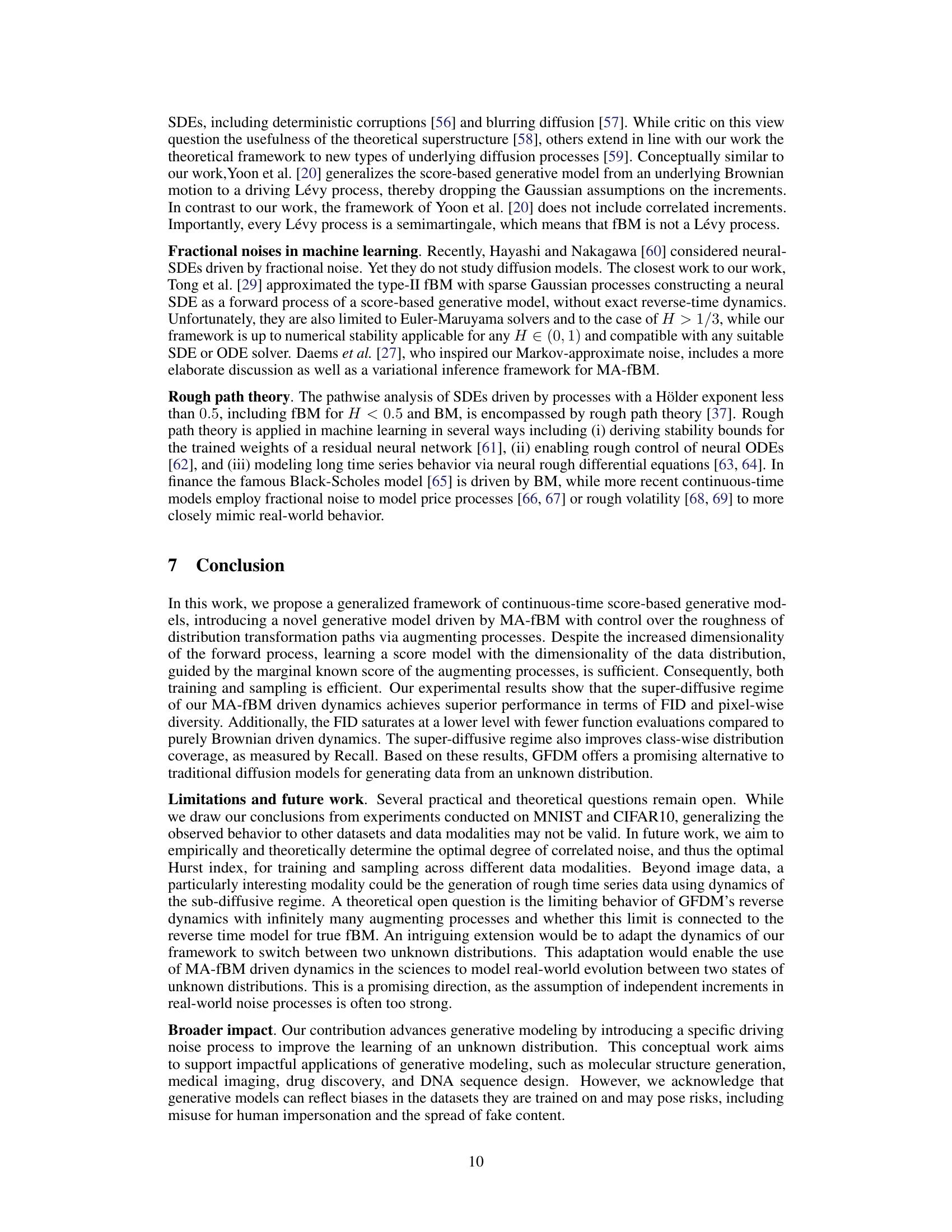
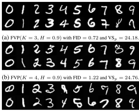
This table compares the performance of the proposed Generative Fractional Diffusion Models (GFDM) against traditional Variance Exploding (VE) and Variance Preserving (VP) diffusion models. It shows the Fréchet Inception Distance (FID) and pixel-wise diversity (VSp) scores for both MNIST and CIFAR10 datasets. The results are broken down by the Hurst index (H) and the number of augmenting processes (K), highlighting that GFDM generally achieves better performance (lower FID and higher VSp), particularly in the super-diffusive regime (H > 0.5).
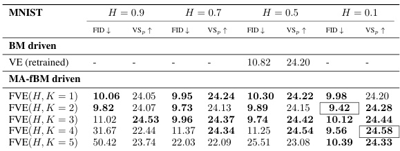
This table compares the Fréchet Inception Distance (FID) and pixel-wise diversity (VSp) scores of Generative Fractional Diffusion Models (GFDM) against traditional Variance Exploding (VE) and Variance Preserving (VP) models using purely Brownian motion. It shows the FID and VSp for different values of the Hurst index (H) and the number of augmenting processes (K). The bold values indicate that the GFDM outperforms both VE and VP. The boxed values represent the overall best scores for each dataset.
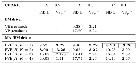
This table presents the results of experiments using Fractional Variance Exploding (FVE) dynamics on the CIFAR10 dataset without Exponential Moving Average (EMA) for training. It compares the performance of the FVE model with different Hurst indices (H) and numbers of augmenting processes (K) against the original Variance Exploding (VE) and Variance Preserving (VP) models using purely Brownian motion. The FID (Fréchet Inception Distance) and VSp (pixel-wise diversity) are reported as metrics to evaluate image quality and diversity respectively. Bold values indicate performance superior to both VE and VP baselines.
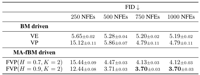
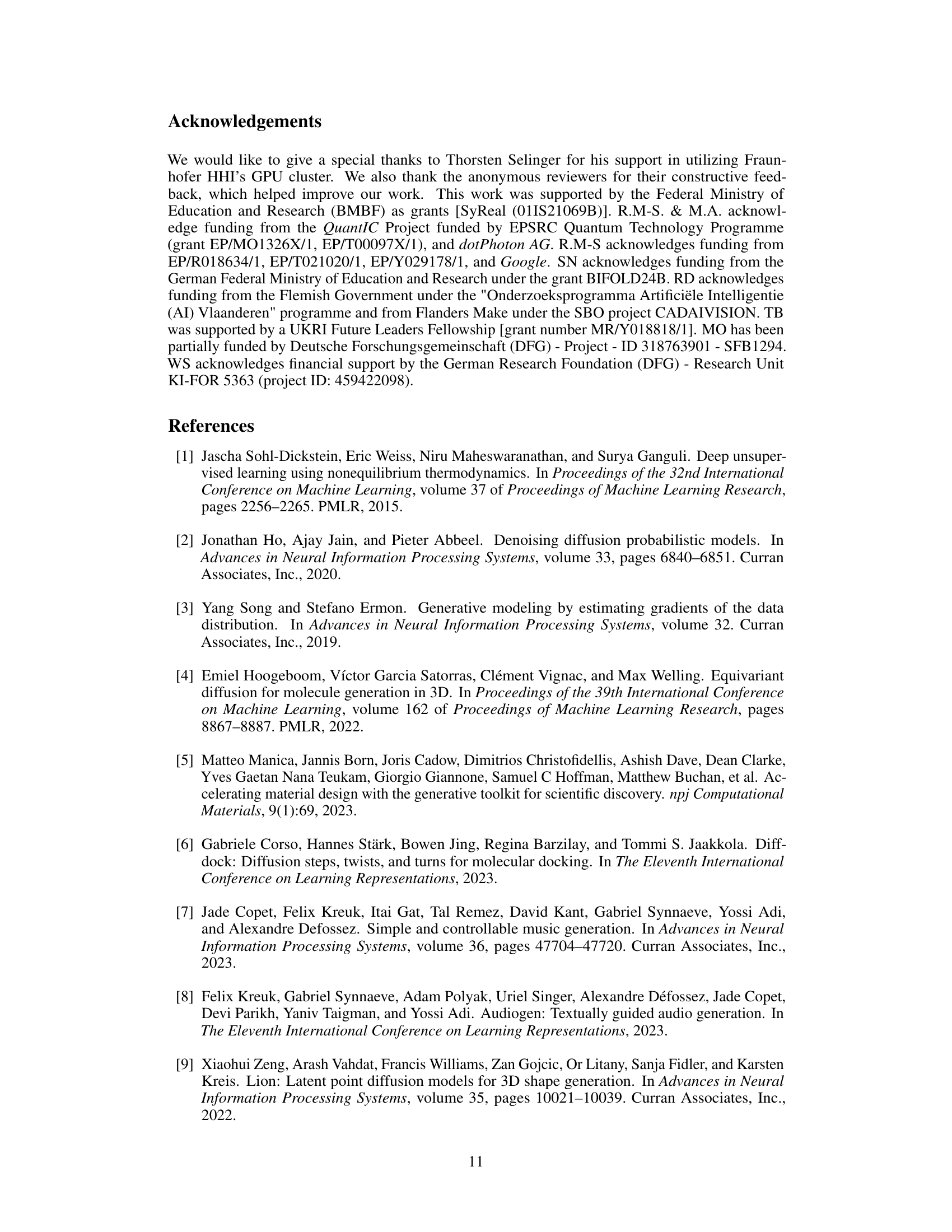
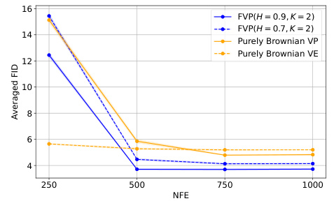
This table compares the FID values obtained using the purely Brownian driven dynamics (VE and VP) against those obtained using the MA-fBM driven dynamics (FVP) with H = 0.7 and H = 0.9, and K = 2. The comparison is done for different numbers of function evaluations (NFEs) (250, 500, 750, and 1000). Lower FID indicates better image quality.

This table shows the average computation time required to calculate the optimal approximation coefficients (ω₁, …, ωκ) for different values of K (number of augmenting processes) before the training process begins. The computation time is measured in seconds and obtained using a GPU Tesla V100 with 32 GB of RAM. The Hurst index H was randomly sampled 1000 times from a uniform distribution between 0.1 and 0.9 for each K.

This table shows the average computation time for one training step using FVE dynamics on the CIFAR10 dataset. The experiment uses a conditional U-Net with approximately 58.7 million parameters and exponential moving average (EMA) for training. The batch size is 128. The table breaks down the average time for different Hurst indices (H) and numbers of augmenting processes (K).

This table shows the average computation time for a single training step using the Fractional Variance Exploding (FVE) dynamics on the CIFAR10 dataset. The experiment uses a conditional U-Net architecture with approximately 58.7 million parameters and Exponential Moving Average (EMA) for model training. The batch size was 128. The results are broken down by Hurst index (H) values of 0.9, 0.5, and 0.1 and include the average across these values. The values represent the average time across multiple training steps.

This table shows the average time it takes to perform one sampling step in the reverse dynamics of the Fractional Variance Exploding (FVE) model for different Hurst exponents (H) and numbers of augmenting processes (K). The experiment uses a conditional U-Net with 58.7 million parameters and exponential moving average (EMA). The batch size is 1000. The data dimensionality is 3x32x32.

This table shows the impact of increasing the number of augmenting processes (K) on the quality and diversity of generated images from MNIST dataset. Two different dynamics, Fractional Variance Exploding (FVE) and Fractional Variance Preserving (FVP), are compared, and the results are evaluated using FID (Fréchet Inception Distance), NLLs (negative log-likelihoods of test data), and VSp (pixel Vendi Score). For each combination of dynamics (FVE or FVP) and number of augmenting processes (K=1 to 5), the table shows the FID, NLLs, and VSp metrics. Lower FID values indicate better image quality, lower NLLs values indicate better model fit, and higher VSp values indicate better pixel-wise diversity.
Full paper#
