Efficiently Learning Significant Fourier Feature Pairs for Statistical Independence Testing

↗ OpenReview ↗ NeurIPS Homepage ↗ Chat

TL;DR

#

Key Takeaways

#

Why does it matter?

#

This paper is crucial for researchers working on independence testing, particularly those dealing with high-dimensional data. It offers a novel, efficient method that significantly improves the power and speed of existing techniques, opening avenues for applications in causal inference, feature selection, and deep learning. The theoretical foundation provided is also valuable for further advancements in the field.

Visual Insights

#

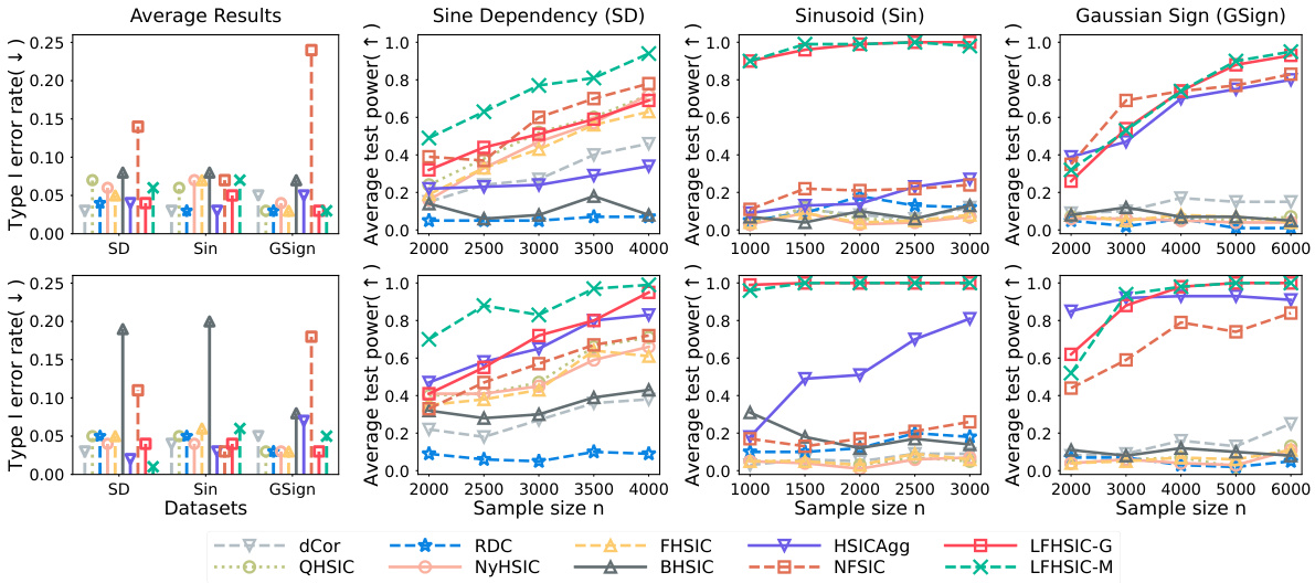
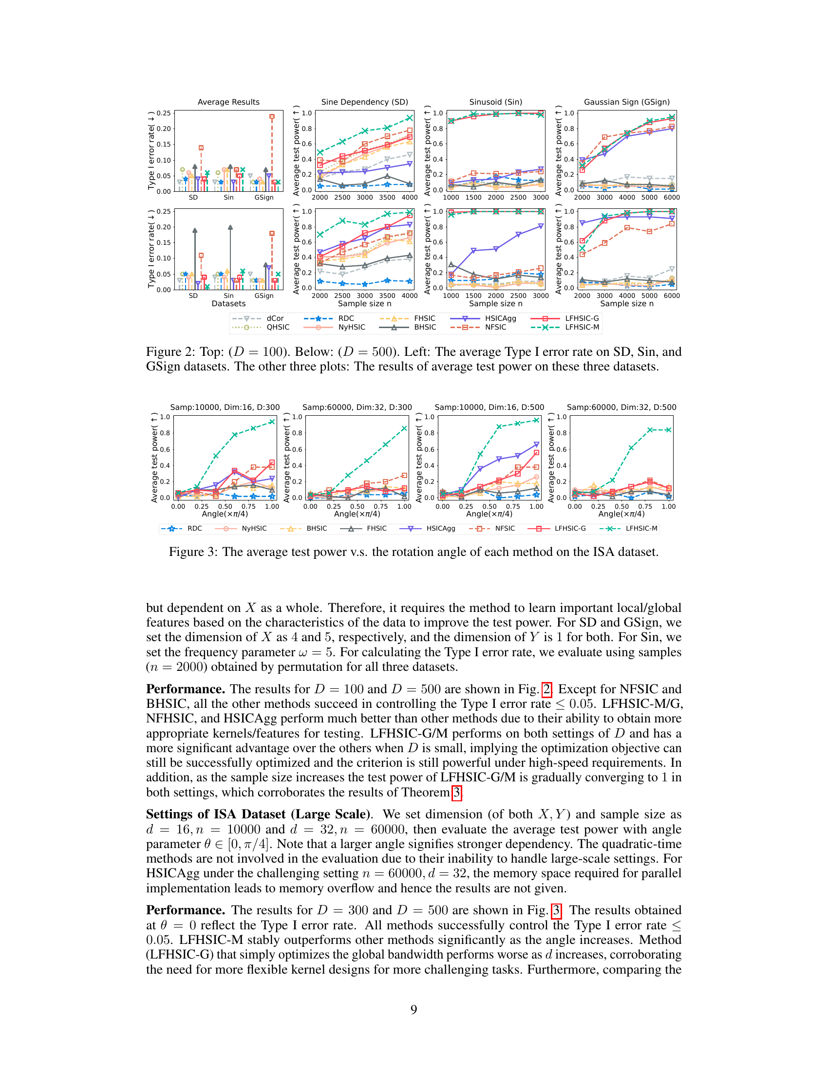
This figure shows the results of the average Type I error rate and average test power for different sample sizes on three synthetic datasets: Sine Dependency (SD), Sinusoid (Sin), and Gaussian Sign (GSign). The top row displays results with D=100 Fourier features, while the bottom row shows results with D=500. The leftmost plot compares Type I error rates across different methods and datasets. The remaining plots present the average test power for each dataset, showcasing how the power changes with the sample size and the different methods used.

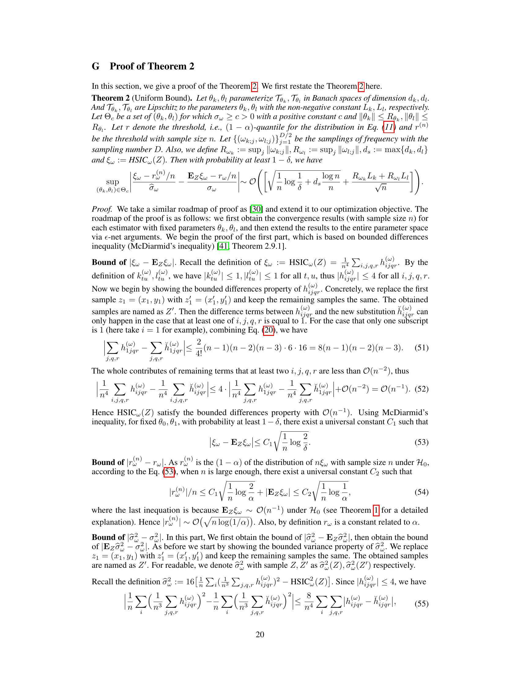
This table lists some commonly used kernels and their corresponding density functions in the frequency domain. The kernels are parameterized by σ (sigma) and Σ (Sigma), representing the bandwidth and covariance matrix, respectively. The inverse Fourier transforms of these kernels are also provided, showing the probability density functions in the frequency domain used for sampling in the Random Fourier Features (RFF) approach.

In-depth insights

#

HSIC Frequency View

#

The heading ‘HSIC Frequency View’ suggests an analysis of the Hilbert-Schmidt Independence Criterion (HSIC) from a frequency domain perspective. This approach likely involves transforming the data using Fourier transforms to represent it in the frequency domain, then applying HSIC to these transformed representations. This frequency-based interpretation offers several potential advantages: it could reveal hidden dependencies not apparent in the time domain; provide a more intuitive understanding of HSIC’s behavior by linking it to the frequency content of the data; and potentially lead to more efficient computational methods by focusing on only the most significant frequency components. A key insight might be the identification of specific frequency ranges or bands that contribute most significantly to the dependence measure. This could enable improved feature selection or more powerful independence testing by selectively focusing on those frequency bands. Conversely, a frequency-based analysis might reveal limitations in HSIC’s ability to capture certain types of dependencies that might be manifested in specific frequency patterns. Understanding these aspects of the ‘HSIC Frequency View’ can help optimize the performance of HSIC and broaden its applicability in various domains.

Learnable Fourier Pairs

#

The concept of “learnable Fourier pairs” presents a powerful advancement in statistical independence testing. By moving beyond fixed kernel methods, this approach uses machine learning to optimize the Fourier features employed in the Hilbert-Schmidt Independence Criterion (HSIC). This dynamic adaptation allows the test to focus on the most discriminative frequency components specific to the data, significantly boosting its power, especially when dealing with complex, high-dimensional data. The learnability of these features means the method can flexibly adjust to diverse data distributions, unlike traditional methods constrained by inflexible configurations. Furthermore, the framework’s linear time complexity makes it computationally efficient for large-scale data analysis, providing a significant practical advantage. This approach bridges the gap between the theoretical power of HSIC and the computational demands of real-world applications, offering a substantial improvement in both effectiveness and efficiency.

Linear Time Learning

#

Linear time learning algorithms are crucial for handling large-scale datasets. The core idea is to design algorithms whose computational complexity scales linearly with the size of the input data, i.e., O(n), where n is the number of data points. This contrasts sharply with algorithms having quadratic (O(n²)) or cubic (O(n³)) complexity, which become computationally infeasible for massive datasets. The significance of linear time learning lies in its ability to maintain efficiency and scalability even with an explosion in data size. Such algorithms often employ clever techniques like randomized projections, approximate nearest neighbor searches, or divide-and-conquer strategies to achieve linear scaling. A key challenge in designing linear time learning methods is to trade off the reduction in computational complexity with accuracy and performance. Finding the optimal balance is crucial. Successful linear time learning approaches often involve careful approximations that preserve the essential information while discarding less relevant details, resulting in speed-ups without sacrificing too much accuracy. This makes the development of robust and accurate linear-time learning algorithms an active area of research in machine learning and data science.

Theoretical Guarantees

#

A theoretical guarantees section in a machine learning research paper would rigorously establish the soundness and reliability of the proposed method. It would likely involve proving convergence results, showing that the algorithm’s output approaches the desired solution as the number of iterations or data points increases. Additionally, it might involve demonstrating generalization bounds, which quantify how well the model is expected to perform on unseen data based on its performance on the training data. Consistency proofs would also be crucial, asserting that the model’s predictions converge to the true underlying relationship as the sample size grows. The analysis would likely include non-asymptotic bounds, which provide finite-sample guarantees, and may leverage tools from statistical learning theory, such as Rademacher complexity or VC-dimension. The complexity of the analysis would heavily depend on the algorithm’s specifics and the problem setting, with simpler algorithms potentially allowing for tighter and more easily interpretable guarantees. Successfully establishing these theoretical guarantees builds trust and confidence in the method’s reliability and efficacy beyond empirical observations.

High-Dim Experiments

#

In high-dimensional settings, the challenges of independence testing are amplified due to the curse of dimensionality. A key consideration in evaluating a method’s effectiveness is its performance on high-dimensional data, as this often reveals limitations of methods that are effective in lower dimensions. High-dimensional experiments should thoroughly assess a test’s power and type I error control across a range of dimensionality. Synthetic datasets, with controlled dependencies and varying dimensionality, are invaluable for establishing the method’s behavior and validating theoretical claims. Real-world datasets are equally crucial for demonstrating the method’s practicality on complex, high-dimensional data structures that capture real-world complexities. A comparative analysis against existing methods is crucial, providing a contextualized performance evaluation. The choice of metrics—such as power, Type I error, and runtime—should reflect both statistical and computational aspects for practical considerations. Finally, it’s important to consider potential overfitting or underfitting in high dimensions, investigating the impact of the method’s hyperparameters and the sample size.

More visual insights

#

More on figures

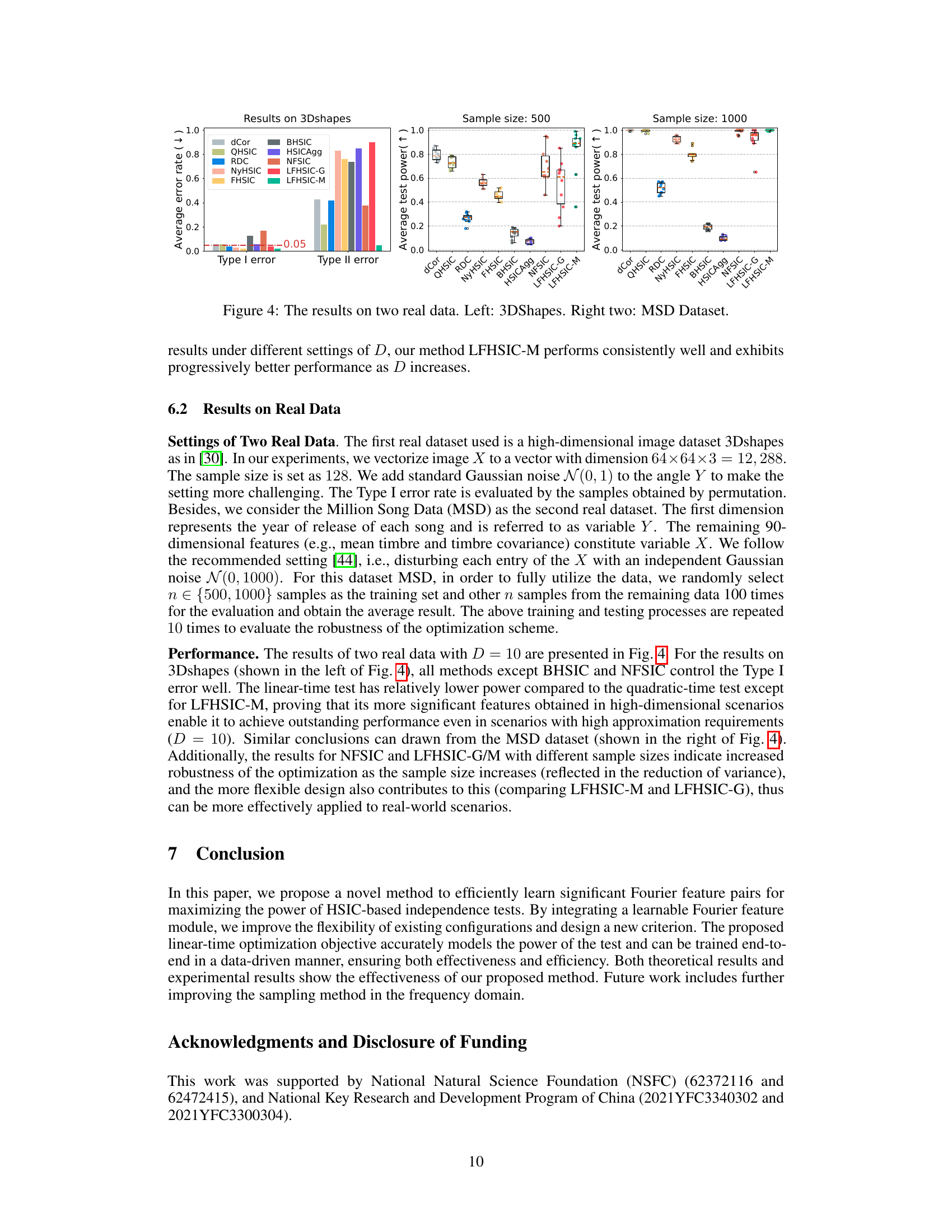
This figure shows the average test power of various independence tests against the rotation angle in the ISA dataset. The rotation angle represents the dependency between variables X and Y. A larger angle means stronger dependence. The figure demonstrates the performance of different methods in detecting dependencies at various levels of dependency strength, allowing comparison of their ability to capture non-linear relationships.

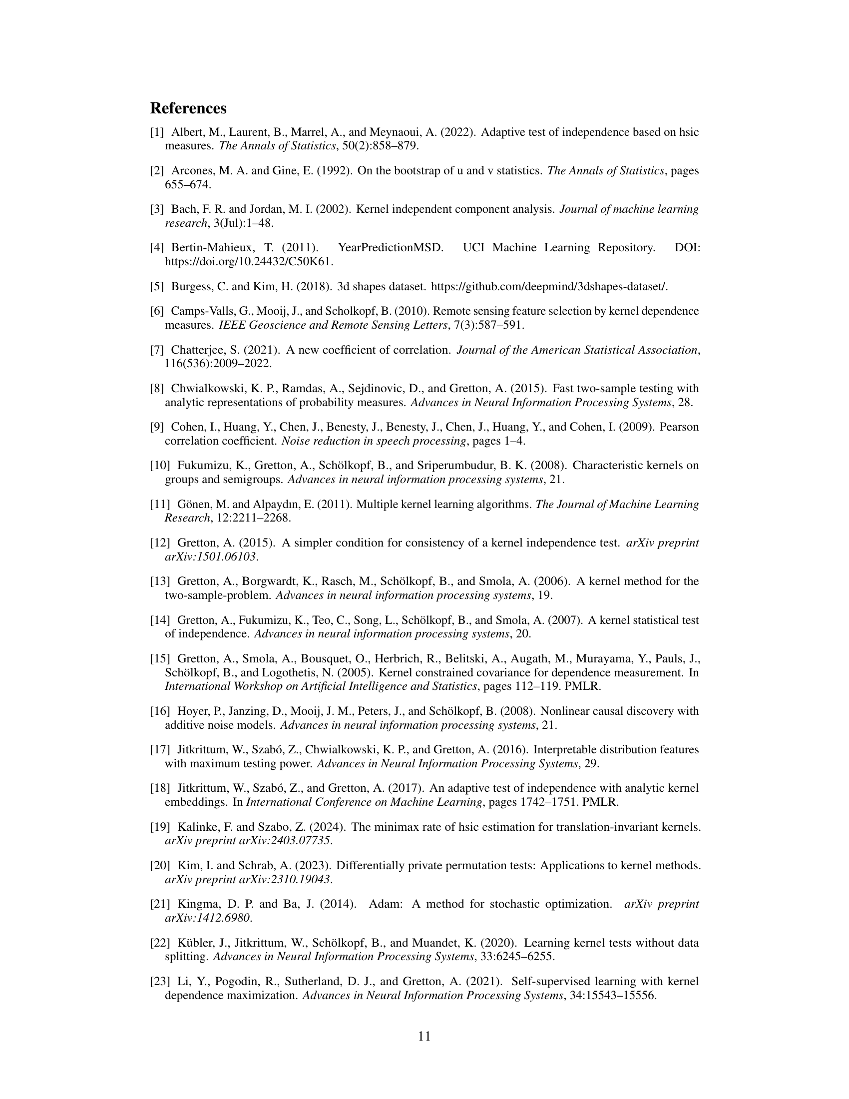
This figure shows the results of applying different methods to two real datasets: 3DShapes and Million Song Dataset (MSD). The leftmost panel displays average Type I and Type II error rates for various methods on the 3DShapes dataset. The other two panels present boxplots of the average test power for each method on MSD for sample sizes of 500 and 1000, respectively. The plots compare the performance of the proposed method (LFHSIC-G/M) against existing methods, demonstrating its effectiveness in real-world scenarios.

This figure visualizes samples from three different datasets used in the paper: Sin, ISA, and 3DShapes. The leftmost panel shows a contour plot of samples from the Sin dataset, illustrating the sinusoidal relationship between X and Y. The middle panel shows samples from the ISA dataset, where the angle parameter θ controls the degree of dependency between X and Y. The rightmost panel provides a causal diagram and sample images from the 3DShapes dataset, showing the dependency between image features (X) and orientation (Y). These visualizations help illustrate the types of relationships the paper’s methods are designed to detect.

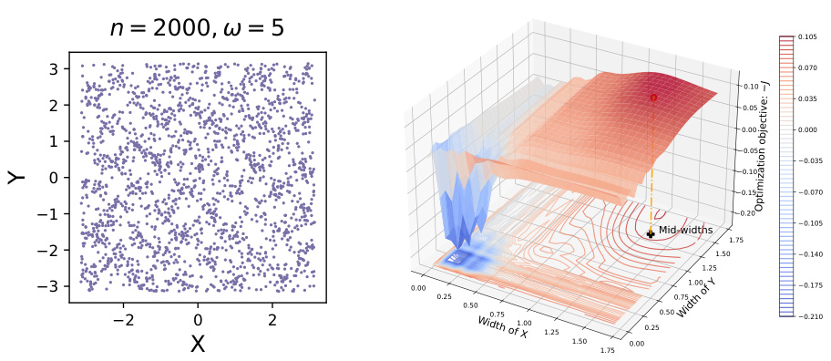
This figure visualizes the performance of the optimization objective used in the paper. The left panel shows a scatter plot of the synthetic Sin dataset used for testing. The right panel displays a 3D surface plot and contour plot of the negative optimization objective, illustrating the relationship between the test power (vertical axis) and the bandwidth parameters for X and Y (horizontal axes). The red dot marks the optimal solution that maximizes test power, aligning with the theoretical analysis. The plot shows how this optimization objective guides the bandwidth to adapt and improve test power, and that this optimization is smooth.

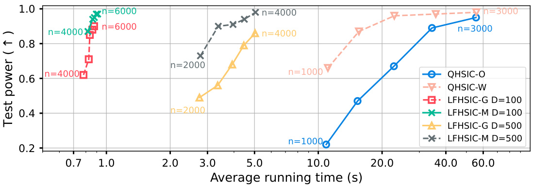
This figure compares the performance of various methods in terms of test power and average running time on the Sine Dependency (SD) dataset. It showcases the trade-off between efficiency (runtime) and effectiveness (test power) for different sample sizes (n). The results highlight that the proposed LFHSIC-G/M methods achieve a better balance between test power and computational cost compared to other approaches, especially when considering larger sample sizes.

The figure shows the runtime comparison of different independence tests on the ISA dataset with dimensionality d=10. The left panel compares the linear-time methods (O(n) and O(nlogn)), while the right panel shows the runtime of both linear and quadratic (O(n^2)) methods. The x-axis represents the sample size (n), and the y-axis represents the running time in seconds. This visualization highlights the scalability of linear-time methods for large datasets compared to quadratic-time methods.

Full paper

#