Contracting with a Learning Agent

↗ OpenReview ↗ NeurIPS Homepage ↗ Chat

TL;DR

#

Key Takeaways

#

Why does it matter?

#

This paper is crucial because it bridges the gap between theoretical contract design and real-world scenarios involving learning agents. This is highly relevant given the increasing use of AI in various applications where interactions are dynamic and uncertain. The findings offer new insights into designing efficient and beneficial contracts in these complex settings, paving the way for future research and practical applications.

Visual Insights

#

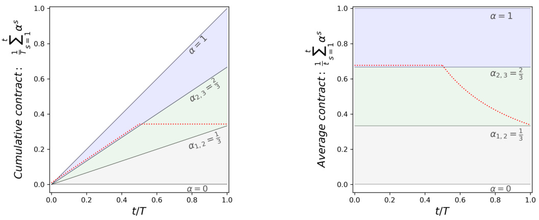
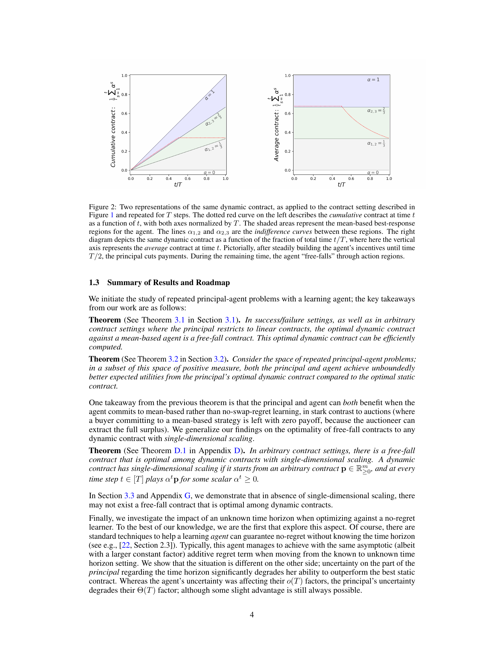
This figure shows two different ways of visualizing the same dynamic contract. The left panel displays the cumulative contract value over time, while the right panel shows the average contract value as a function of the time elapsed (t/T). Both plots illustrate how the principal initially increases the contract value to incentivize the agent towards a specific action, and then abruptly switches to a zero-value contract, causing the agent’s actions to ‘free-fall’ through the action space.

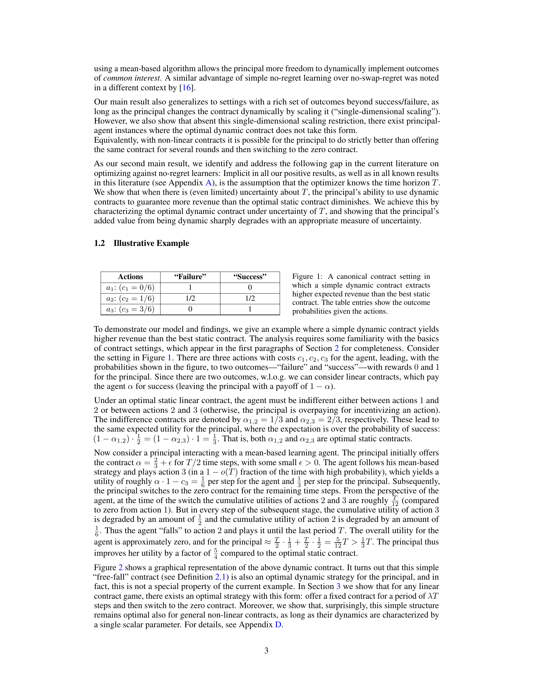
This table presents a canonical contract setting with three actions (a1, a2, a3) and two outcomes (‘Failure’, ‘Success’). Each action has an associated cost (c1, c2, c3) and a probability distribution over the two outcomes. For example, action a1 (with cost 0) results in ‘Failure’ with probability 1 and ‘Success’ with probability 0. Action a3 (with cost 3/6) results in ‘Failure’ with probability 0 and ‘Success’ with probability 1. This setting is used to illustrate how a dynamic contract can outperform the best static contract by strategically changing the contract over time.

In-depth insights

#

Repeated Contracts

#

The concept of ‘Repeated Contracts’ in the context of a research paper likely explores the dynamics of principal-agent interactions over multiple periods. A key aspect would be the evolution of strategies adopted by both the principal (e.g., a firm) and the agent (e.g., a worker or supplier) as they learn from past interactions. This introduces learning algorithms and the influence of uncertainty about the agent’s behavior and the outcome of actions. The paper likely investigates how the optimal contract design might vary in this repeated setting, compared to a single-shot interaction, potentially including the consideration of dynamic contracts that adapt over time. Furthermore, the study may address challenges like moral hazard and information asymmetry, which become more pronounced in repeated scenarios. A key question addressed might be under what conditions a dynamic contract can improve the outcome for both the principal and the agent compared to the best static contract. The research is likely to be theoretically grounded, potentially focusing on mathematical models and game-theoretic analysis. The authors may compare the performance of different types of contracts, considering various learning algorithms that the agent might use.

Learning Agents

#

The concept of ‘Learning Agents’ within the context of a research paper likely explores the intersection of artificial intelligence and game theory, specifically focusing on how agents adapt and learn within dynamic environments. A core aspect is the agents’ ability to modify their strategies over time based on past experiences, potentially involving reinforcement learning, multi-agent systems, or other machine learning techniques. This adaptive behavior fundamentally changes the nature of the interactions, shifting from static, one-shot games to more complex, repeated interactions. The study likely examines how such learning affects the overall outcome of the game, focusing on efficiency, fairness, convergence to equilibria, and the strategic implications for all participants. Key considerations might include the type of learning algorithm used, the information available to the agents, and the presence of uncertainty or incomplete information. Analyzing the performance of these learning agents against optimal strategies or other learning algorithms provides valuable insights into their effectiveness and limitations, particularly in the design of contracts or mechanisms where agents are incentivized to act in specific ways. The research could explore the conditions under which learning agents achieve desirable outcomes, such as Pareto efficiency, and the ways in which their behavior deviates from perfectly rational agents. Ultimately, a deeper understanding of ‘Learning Agents’ is crucial for developing robust and adaptable AI systems that can function effectively in dynamic and complex environments.

Dynamic Contracts

#

The concept of dynamic contracts, in the context of principal-agent interactions with learning agents, presents a compelling departure from traditional static contract models. Dynamic contracts allow the principal to adjust contract terms over time, adapting to the agent’s learning behavior and potentially achieving better outcomes than with a fixed contract. The study of dynamic contracts necessitates a careful consideration of the agent’s learning algorithm, as different algorithms may respond differently to changing incentives. Mean-based learning algorithms, in particular, have proven amenable to analysis but also reveal a fascinating trade-off: while simpler than no-swap regret learning, they offer the principal greater flexibility in manipulating outcomes. The authors’ work demonstrates that under specific conditions, dynamic contracts can lead to Pareto improvements, benefiting both principal and agent compared to the optimal static contract. This highlights the potential for significant welfare gains through dynamic mechanisms. However, uncertainty about the time horizon significantly complicates the design of optimal dynamic contracts, revealing a trade-off between the potential for increased revenue and the robustness to uncertainty.

Welfare Analysis

#

A welfare analysis in a principal-agent model with learning agents would delve into how the proposed contracting mechanisms impact the overall welfare of both parties. It would be crucial to compare the welfare under dynamic contracts to that under static contracts, considering scenarios where the principal and agent have differing preferences. A key aspect would be to identify cases where dynamic contracts lead to Pareto improvements, boosting welfare for both. The analysis should account for the computational costs of implementing dynamic contracts and explore the robustness of welfare outcomes under different learning algorithms and varying levels of uncertainty regarding agent behavior or the time horizon. Further investigation could determine the conditions under which dynamic contracting yields significant welfare gains, potentially exceeding the gains from optimal static contracts, and also examine whether such improvements disproportionately benefit either principal or agent.

Time Horizon

#

The concept of ‘Time Horizon’ in the context of repeated principal-agent interactions with learning agents is crucial. The paper investigates how uncertainty about the time horizon affects the principal’s ability to leverage dynamic contracts. The key insight is that when the time horizon is unknown, the principal’s advantage in using dynamic strategies significantly diminishes. This highlights the critical role of information in principal-agent problems. The assumption of a known time horizon is commonly made in the literature, but this paper demonstrates its substantial impact. While the principal might still gain some utility through dynamic contracts, the benefit decreases with greater uncertainty about the time horizon, suggesting a trade-off between dynamic strategy complexity and information availability. The authors provide the first analysis of this problem, underlining the need for more robust contract designs that can accommodate such uncertainty in real-world applications.

More visual insights

#

More on figures

This figure shows two different ways of visualizing the same dynamic contract. The left plot shows the cumulative contract value over time, illustrating how the contract changes over the interaction. The right plot shows the average contract value as a function of the fraction of total time, providing a different perspective on the contract’s evolution. The shaded regions represent different actions an agent would choose based on the cumulative contract. The plots illustrate the ‘free-fall’ strategy of the principal where, after a period of increasing incentives, the principal reduces the contract to 0, leading to a shift in the agent’s optimal action.

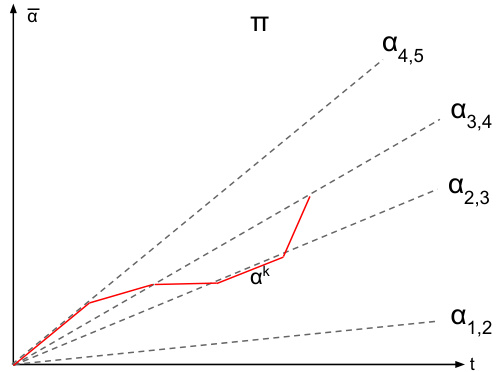
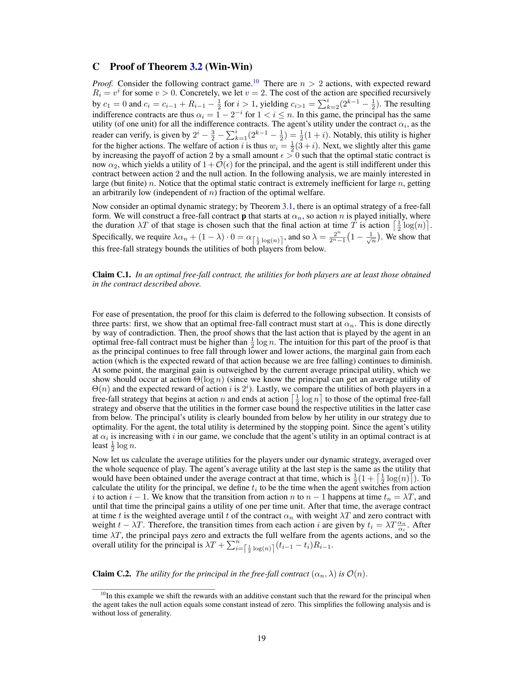
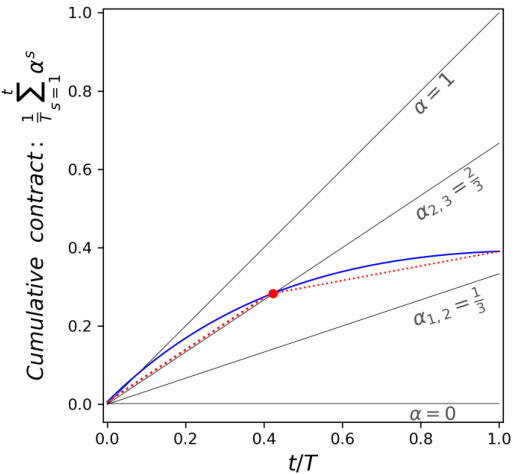
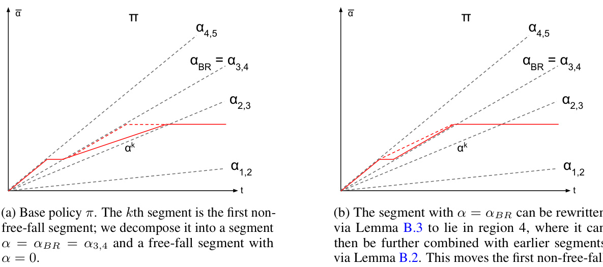
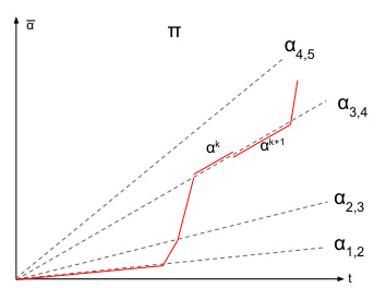
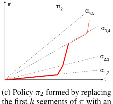
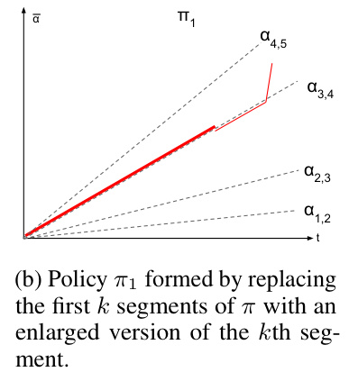
This figure illustrates Lemma B.2, which states that any dynamic contract can be rewritten as a piecewise stationary strategy without changing the agent’s behavior or the principal’s utility. The blue curve represents an arbitrary dynamic contract, while the red dotted curve shows its piecewise stationary equivalent. Both strategies induce the same cumulative contract and agent actions, highlighting the simplification achieved through Lemma B.2.

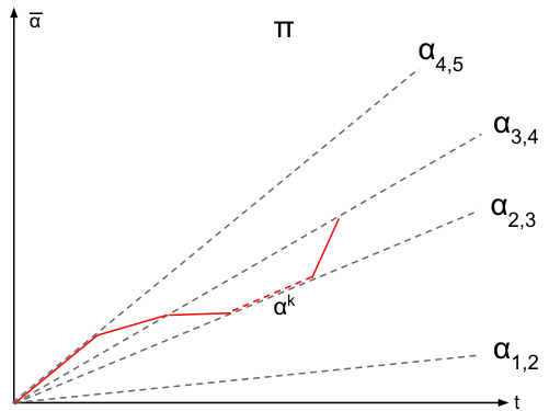
This figure illustrates Lemma B.2, which states that any dynamic contract can be rewritten as a piecewise stationary contract with the same utility. The figure shows a cumulative contract (vertical axis) over time (horizontal axis) for a specific contract game. The blue curve represents an arbitrary dynamic strategy. The lemma shows that this arbitrary dynamic strategy can be rewritten into a piecewise stationary strategy, represented by the dotted red curve, yielding the same utilities for the players.

This figure shows two different ways of visualizing the same dynamic contract applied to the setting in Figure 1. The left panel shows the cumulative contract value over time, normalized by the total number of time steps T. The shaded areas represent the agent’s best response regions to the contract. The dotted red line shows an optimal dynamic contract strategy where the principal first increases the agent’s incentive and then abruptly reduces it to zero, causing the agent’s actions to ‘free-fall’ towards a lower-cost action. The right panel shows the same dynamic contract as a function of the fraction of total time, clearly illustrating the time at which the principal switches from offering a high incentive contract to a zero-incentive one.

This figure shows two different ways of visualizing the same dynamic contract, which consists of a linear contract with a high α value for the first half of the time horizon, followed by a zero contract for the second half. The left panel shows the cumulative contract value over time, while the right panel shows the average contract value as a function of the fraction of the time horizon. The shaded regions illustrate the agent’s best-response actions under the mean-based learning model, with the lines α1,2 and α2,3 indicating indifference points between different actions. The dynamic contract is designed to initially incentivize the agent to take a costly action that yields a high reward, and then to switch to a less costly action when the incentives are removed, resulting in a higher total payoff for the principal.

This figure shows two different visualizations of the same dynamic contract applied over T time steps. The left panel displays the cumulative contract value over time, revealing how the contract changes over T time steps. The shaded regions represent the best-response areas for a mean-based learning agent, and the lines indicate indifference points between the action choices. The right panel presents an alternative view of this contract, showing how the average contract changes as a function of the percentage of total time elapsed, illustrating the principal’s strategy of initially incentivizing the agent and then reducing payments to encourage specific actions.

This figure shows two different ways to represent a dynamic contract. The left panel shows the cumulative contract value over time, normalized by the total time horizon T. The shaded regions show the best response for a mean-based agent, and the lines show indifference points. The right panel shows the same contract, but this time it shows the average contract value at time t, normalized by T. This figure illustrates how the principal incentivizes the agent by increasing the contract up to T/2 and then rapidly decreasing it to zero for the remaining half of the period, thereby exploiting the agent’s mean-based strategy.

The figure shows two different visualizations of the same dynamic contract, applied to a specific contract setting. The left panel displays the cumulative contract value over time, highlighting the best-response regions for the agent and indifference curves. The right panel shows the average contract value as a function of the time elapsed. The contract design involves steadily increasing the agent’s incentive until a certain point, after which the principal cuts payments, causing the agent’s actions to shift.

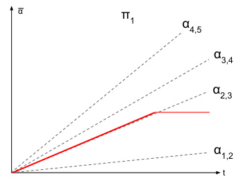
This figure shows two different ways to visualize the same dynamic contract, applied to a repeated game setting. The left panel displays the cumulative contract value over time, normalized by the total time horizon T, showing how the contract increases initially and then drops to zero. The shaded regions show the best response regions for the agent, while the lines α1,2 and α2,3 indicate the indifference curves. The right panel presents the average contract value as a function of the fraction of total time, providing another perspective on the contract’s evolution. The contract gradually increases incentives until half the time horizon and then sharply declines to zero, causing the agent to transition to lower-cost actions.

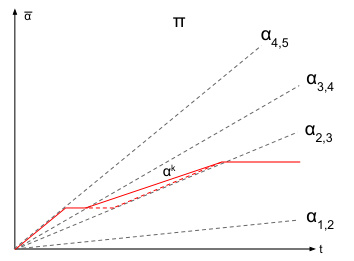
This figure shows two different ways to represent the same dynamic contract. The left panel shows the cumulative contract over time. The shaded regions represent the best response of the mean-based agent. The right panel shows the average contract as a function of the fraction of total time. The contract starts with steadily increasing incentives to the agent, then switches to zero, making the agent’s best response ‘free-fall’ through the action space.

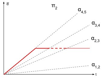
This figure shows two different ways of visualizing the same dynamic contract. The left panel shows the cumulative contract value over time, while the right panel shows the average contract value over time as a fraction of the total time horizon. Both visualizations highlight the key feature of the dynamic contract: a period of increasing incentives followed by a period where the agent’s reward drops to zero, causing the agent to shift actions. The shaded regions in the left panel represent the regions where the agent’s best response is a specific action.

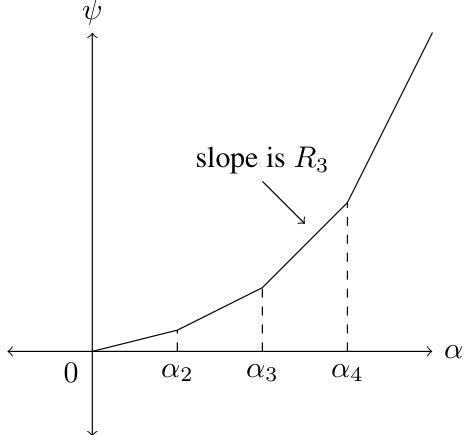
This figure shows a piecewise linear function ψ(α), representing the ‘raw’ potential. The x-axis represents the time-averaged linear contract α, ranging from 0 to α4. The y-axis represents the potential ψ(α). The function is piecewise linear, with different slopes between the breakpoints α2, α3, and α4. The slope between α3 and α4 is explicitly labeled as R3, indicating the expected reward associated with action 3. This function maps the time-averaged linear contract to a potential value; it serves as a tool in the mathematical proof within the paper to analyze the principal’s ability to extract additional profit by gradually lowering their time-averaged linear contract.

Full paper

#