↗ OpenReview ↗ NeurIPS Homepage ↗ Hugging Face ↗ Chat
TL;DR#
Scaling up the number of experts in Mixture of Experts (MoE) models is crucial for achieving fine-grained specialization, but it comes with a high computational cost. Existing sparse MoEs also suffer from training instability and expert underutilization issues. This research proposes a new layer called the Multilinear Mixture of Experts (μMoE) layer to address these challenges.
The μMoE layer uses tensor factorization to perform implicit computations on large weight tensors, resulting in significant improvements in both parameter and computational efficiency. The researchers demonstrate that μMoEs achieve increased expert specialization and enable manual bias correction in vision tasks. They also show that μMoEs can be used for pre-training large-scale vision and language models, maintaining comparable accuracy to those using traditional MLPs, all while offering enhanced interpretability.
Key Takeaways#
Why does it matter?#
This paper is crucial for researchers in deep learning and computer vision due to its novel approach to scaling Mixture of Experts (MoE) models. It addresses the computational challenges of large-scale MoEs by introducing a factorized model, leading to improved efficiency and interpretability. The findings on expert specialization and bias correction offer practical guidance, while the successful pre-training of large models with MoE layers opens new avenues for research in model scalability and interpretability.
Visual Insights#
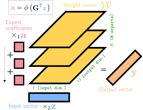
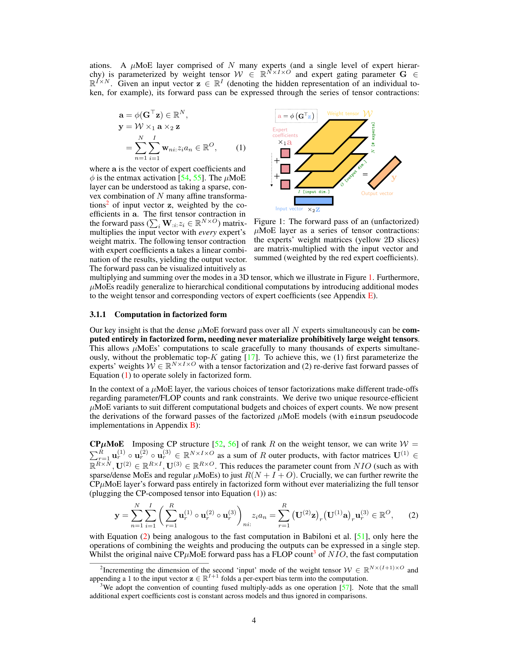
This figure illustrates the forward pass of a Multilinear Mixture of Experts (µMoE) layer. The input vector is first multiplied with each expert’s weight matrix. The resulting vectors are then weighted by the expert coefficients (which are calculated using a gating mechanism) and summed to produce the final output vector. This visualization helps to understand how µMoEs combine multiple expert’s computations to produce a single output.

This table summarizes the advantages of the proposed Multilinear Mixture of Experts (μMoE) model over existing Mixture of Experts (MoE) models. It highlights that μMoEs are differentiable, parameter-efficient, and FLOPs-efficient, unlike dense MoEs which are not parameter or FLOPs efficient, and sparse MoEs which are not differentiable and only parameter efficient.
In-depth insights#
μMoE: Factorised MoE#
The concept of “μMoE: Factorised MoE” presents a novel approach to Mixture of Experts (MoE) models by employing factorization techniques to handle the prohibitively large weight tensors that typically hinder the scalability of MoEs. This factorization allows for implicit computations, thus avoiding the high inference-time costs associated with dense MoEs while simultaneously mitigating the training issues stemming from the discrete expert routing in sparse MoEs. The approach leverages the inherent tendency of experts to specialize in subtasks, offering potential improvements in model interpretability, debuggability, and editability. This is achieved by scaling the number of experts without incurring excessive computational costs during both training and inference. The differentiable nature of the proposed μMoE layer is a significant advantage, ensuring smooth and stable training, in contrast to the non-differentiable nature of the popular sparse MoEs. The use of different tensor factorization methods (like CP and Tensor Ring decomposition) provides flexibility to balance between parameter efficiency and the ability to capture complex interactions in the model.
Expert Specialisation#
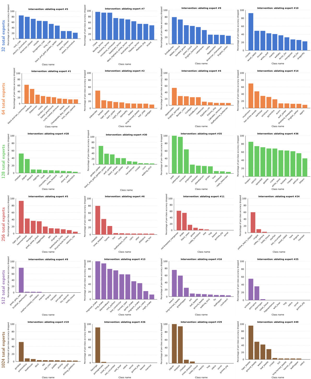
The research explores expert specialization within the Multilinear Mixture of Experts (µMoE) model architecture. Increasing the number of experts leads to more specialized, monosemantic experts, each focusing on a narrower range of input features, as evidenced through qualitative visualizations and quantitative analyses of expert activations and counterfactual interventions. This specialization is beneficial for interpretability, debugging, and editing, allowing for targeted bias mitigation by manually adjusting the contributions of specific experts. The results demonstrate that this improved specialization is not at the expense of model accuracy. Furthermore, µMoEs scale more efficiently than traditional dense or sparse MoEs, avoiding the non-differentiable routing issues associated with sparse models. The ability to achieve high degrees of expert specialization while retaining accuracy and efficiency highlights the potential of µMoEs for creating more explainable and controllable large-scale models.
Bias Mitigation#
The research paper explores bias mitigation within the context of large-scale models, particularly focusing on the Mixture of Experts (MoE) architecture. It highlights how the inherent modularity of MoEs, where individual experts specialize in distinct subtasks, offers a unique opportunity to address bias. The authors demonstrate that scaling the number of experts leads to increased specialization, which in turn facilitates the identification and correction of biased subcomputations. A key contribution is the introduction of a novel method that enables manual bias correction by strategically modifying the weights associated with specific experts. This approach allows for targeted interventions, correcting biased outputs for demographic subpopulations without the need for extensive retraining. The effectiveness of this method is validated through experiments on real-world datasets, showcasing its potential for creating fairer and more equitable AI systems. However, the paper also acknowledges limitations, including the absence of fine-grained labels that would enable a more rigorous evaluation of bias. Furthermore, the paper only evaluates the effectiveness of the bias mitigation techniques at the class level.
Pre-training μMoEs#
Pre-training μMoEs presents a compelling strategy for cultivating specialized experts within large-scale language and vision models. By initializing model layers with μMoE blocks during pre-training, rather than standard MLPs, the network learns a more modular representation. This approach allows individual experts to focus on specific semantic subtasks, leading to improved interpretability and potentially enhanced robustness. The key advantage lies in μMoE’s efficiency in handling vast numbers of experts without incurring prohibitive computational costs, a significant limitation of traditional MoE architectures. Furthermore, the differentiable nature of μMoEs avoids the training instability often associated with sparse MoEs. Pre-training with μMoEs thus offers a pathway to building models with fine-grained, specialized expert knowledge before any downstream fine-tuning, potentially accelerating the adaptation of the models to various downstream tasks. The results demonstrate comparable accuracy with significantly better interpretability, suggesting that pre-training μMoEs is a promising direction for enhancing the scalability and explainability of large language models and vision transformers.
μMoE Limitations#
The core limitation of the proposed multilinear mixture of experts (μMoE) model centers on the qualitative assessment of expert specialism. While quantitative metrics demonstrate improved performance and efficiency, a lack of granular ground truth labels hinders definitive proof of fine-grained expert specialization. The reliance on visualization and counterfactual intervention for evaluating expert behavior means the subjective nature of interpretation remains a significant factor. Furthermore, the current empirical evaluation primarily focuses on model performance using established benchmark datasets. Extending the evaluation to out-of-distribution data and more complex real-world tasks is essential for a comprehensive assessment of μMoE’s capabilities and limitations. Another factor to consider is scalability. While μMoE addresses some scaling issues of existing MoEs, further investigation is required to assess its performance and efficiency when applied to extremely large models with trillions of parameters. Finally, the interpretability benefits, though promising, are largely qualitative. More robust quantitative methods for assessing the level of human-understandable task decomposition are needed to fully confirm the μMoE’s contribution to explainability and transparency.
More visual insights#
More on figures

This figure compares the qualitative results of using CPµMoE layers with 256 and 32 experts, respectively, when fine-tuned on CLIP ViT-B-32. The images displayed show those that had an expert coefficient of at least 0.5. The figure demonstrates that as the number of experts increases, each expert becomes more specialized, focusing on specific visual themes or image categories. In contrast, fewer experts result in experts that process a broader range of image categories.
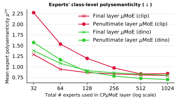
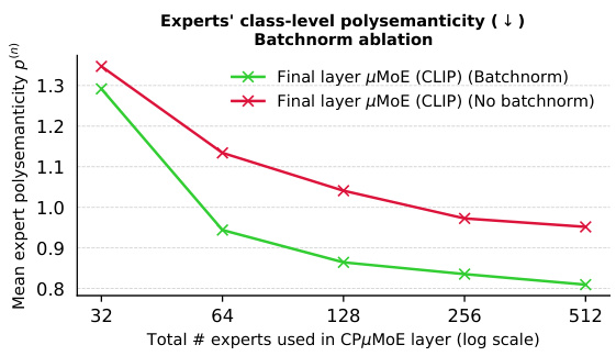
This figure shows the relationship between the number of experts in a CPµMoE layer and the resulting expert specialization. The y-axis represents the mean expert class-level polysemanticity, a measure of how focused each expert is on a single class. The x-axis shows the total number of experts used. The results demonstrate that as the number of experts increases, the experts become more specialized in processing images belonging to specific classes, indicating an improvement in monosemanticity.

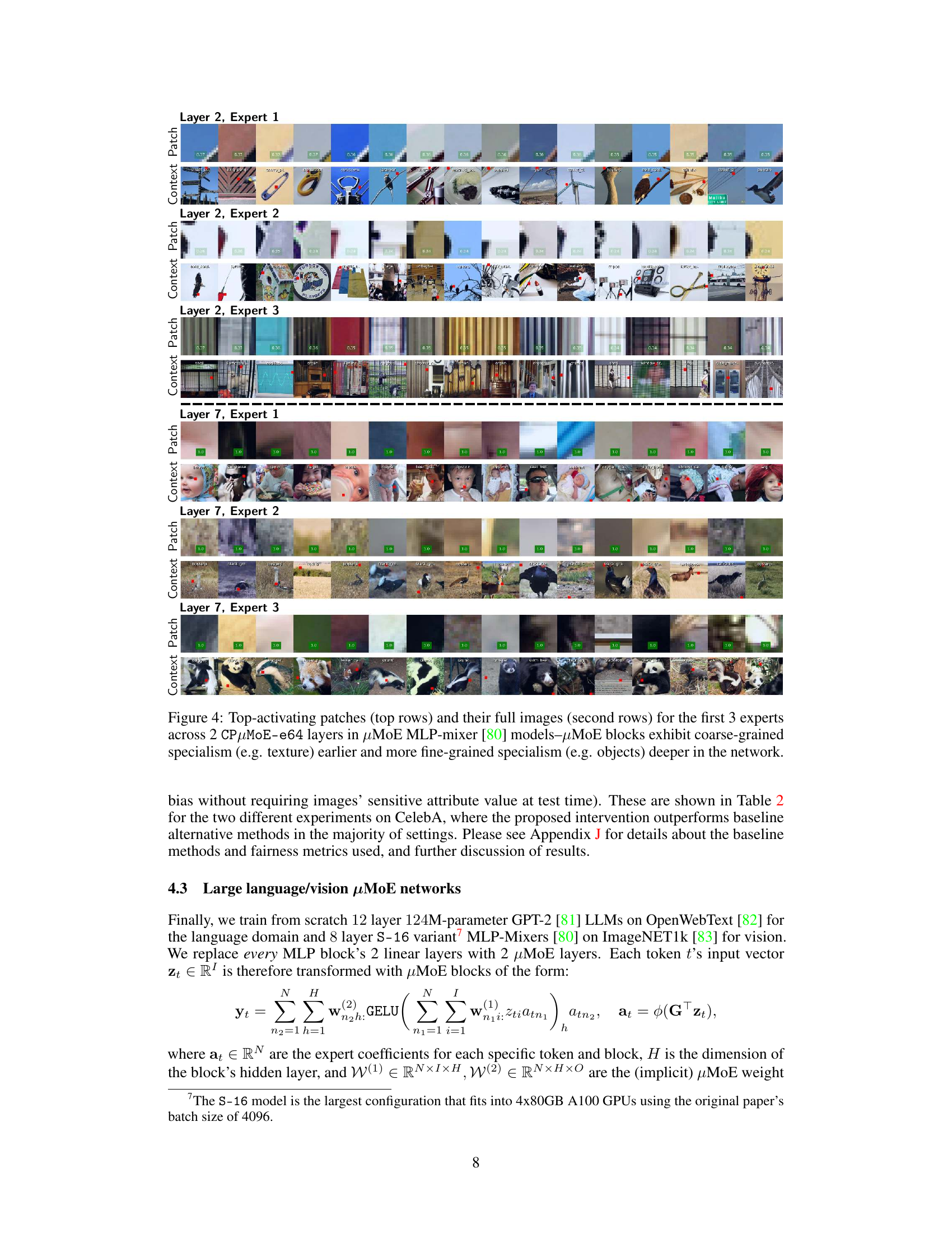
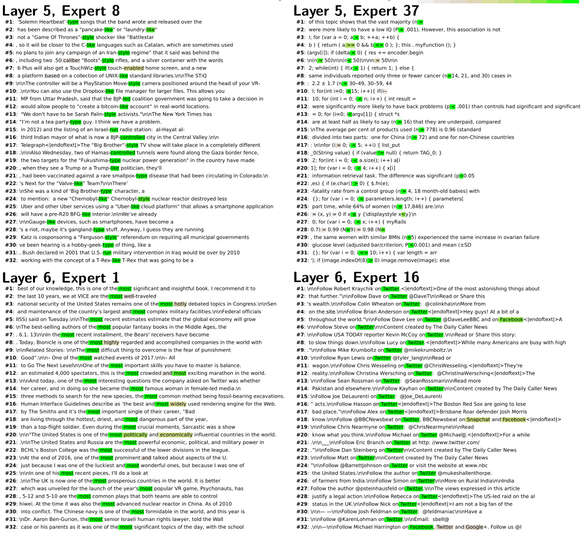
This figure visualizes the top-activating image patches and their corresponding full images for the first three experts across two CPµMoE layers (with 64 experts each) within a µMoE MLP-mixer model. It demonstrates how µMoE blocks develop specializations at different levels of granularity. In the earlier layers (Layer 2), the experts show coarse-grained specialism, focusing on texture. As the network deepens (Layer 7), the experts exhibit more fine-grained specialism, concentrating on object categories.
This figure compares the qualitative results of fine-tuning CLIP ViT-B-32 with CPµMoE layers using 256 and 32 total experts. It shows randomly selected images processed by the first few experts in each model, highlighting the increased specialization observed with a larger number of experts. Experts with 256 total experts show a much stronger tendency to focus on a single visual theme or image category, while experts with 32 total experts tend to exhibit more polysemanticity, processing images from multiple categories.

This figure shows a step-by-step visualization of the unfactorized µMoE forward pass, which is a series of tensor contractions. It illustrates how the output vector is generated by a combination of operations involving the input vector, expert coefficients, and the weight tensor. Each step is visually represented to enhance understanding of the process.
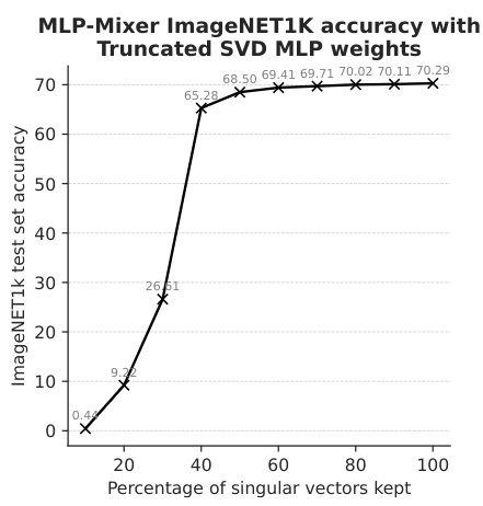
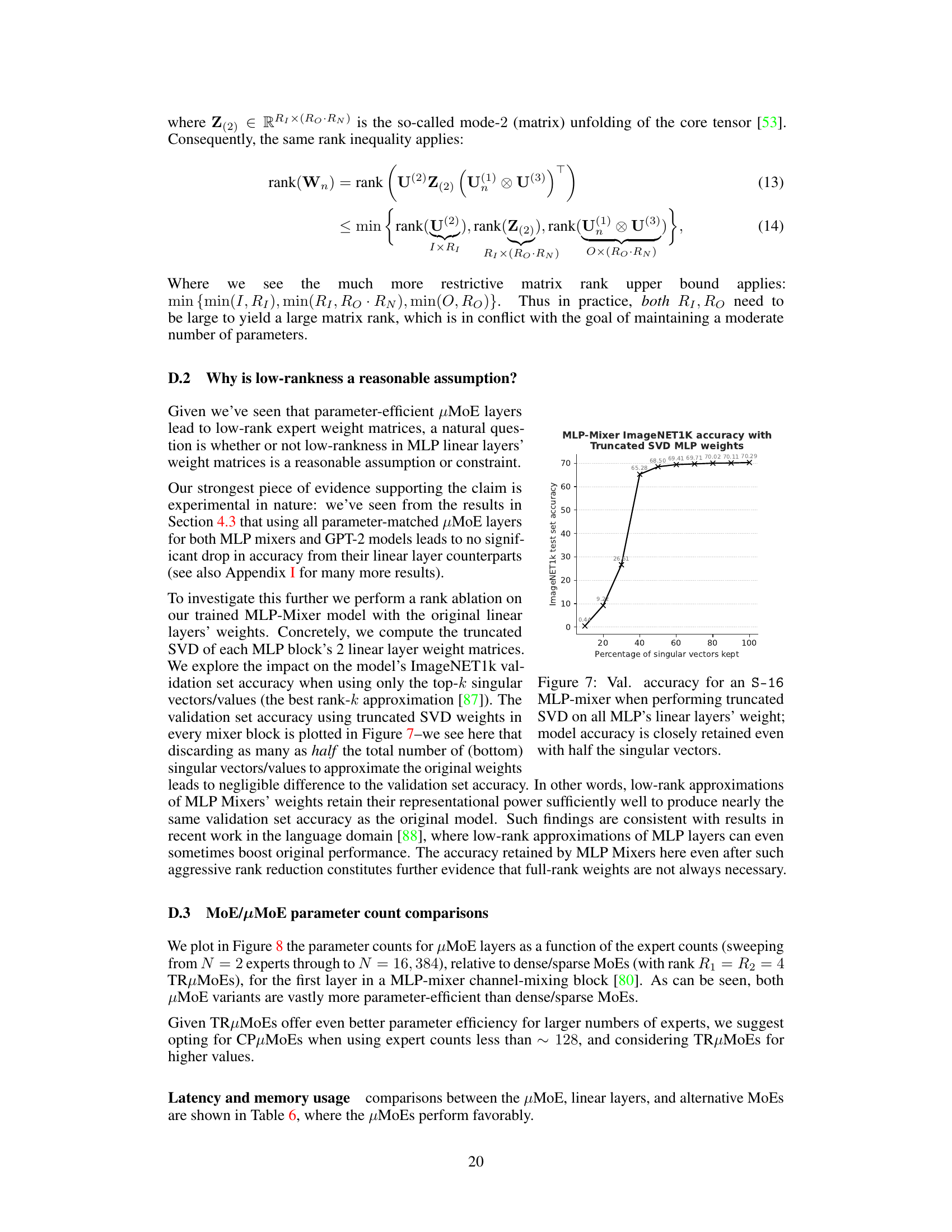
This figure shows the ImageNet1k validation accuracy of an S-16 MLP-Mixer model as a function of the percentage of singular vectors kept after applying truncated Singular Value Decomposition (SVD) to all the model’s linear layers’ weight matrices. The results demonstrate that even when only half of the singular vectors are kept, the model’s accuracy is still very high, suggesting that low-rank approximations of MLP layers in this type of model can be effective.

This figure shows a comparison of the number of parameters required for µMoE layers (CPµMoE and TRµMoE) and traditional sparse/soft MoE layers as a function of the number of experts. The plot demonstrates that µMoE layers, particularly TRµMoE with carefully chosen ranks, require significantly fewer parameters than traditional MoE approaches, especially as the number of experts increases. This highlights the parameter efficiency of the proposed µMoE architecture.
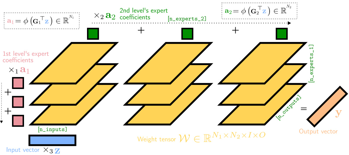
This figure illustrates the forward pass of a two-level hierarchical μMoE layer. It shows how the input vector is processed through a series of tensor contractions involving two sets of expert coefficients (a1 and a2) and the weight tensor W. The visualization helps understand how the layer combines computations from multiple experts at different hierarchical levels to produce the final output vector.
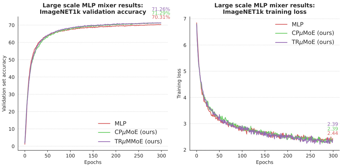
This figure shows the training and validation accuracy curves for MLP-Mixer models trained for 300 epochs. Three different model configurations are compared: a standard MLP model and two versions using the proposed µMoE layers (CPµMoE and TRµMoE). The graphs illustrate the convergence of training loss and the performance on the validation set for each model. This visual comparison allows assessing the training stability and effectiveness of µMoE layers compared to standard MLPs.

This figure shows the training and validation loss curves for MLP-mixer models trained for 300 epochs. The curves represent the performance of three different model variations: a standard MLP, a CPµMoE model, and a TRµMoE model. The plot visually compares the training and validation performance of these models across different epochs, illustrating the convergence of each model’s loss and the accuracy achieved on a validation set. The specific values for the loss and accuracy at the end of training (300 epochs) are shown in a legend box.

This figure shows the top-activating image patches for the first two experts at two different μMoE blocks within MLP-mixer models. The visualization demonstrates how the µMoE blocks learn to specialize in different aspects of the image. Earlier layers show more coarse-grained specialization (texture), while deeper layers show more fine-grained specialization (object category). This provides visual evidence for the claim that increasing the number of μMoE experts leads to increased task modularity and specialization.

This figure shows the top-activating image patches for the first two experts at two different layers in a MLP-mixer model. The model uses μMoE (Mixture of Experts) blocks with 64 experts. The results demonstrate that early layers show coarse-grained specialization (such as texture), while deeper layers demonstrate finer-grained specialization (such as object category).

This figure shows a comparison of expert specialization in two CPµMoE models with different numbers of experts (256 and 32) fine-tuned on the CLIP ViT-B-32 model. Each row presents a subset of images that had activation coefficients of 0.5 or greater for a few experts in each model. The figure demonstrates that increasing the number of experts leads to more specialized experts, where each expert focuses on a narrower set of visual themes or image categories.

This figure shows a comparison of expert specialization in two CPµMoE models fine-tuned on CLIP ViT-B-32, one with 256 experts and the other with 32 experts. Each row displays examples of images processed by a subset of the experts, highlighting the increased specialization of experts in the model with a larger number of experts. The images are selected based on having an expert coefficient of at least 0.5, indicating a strong contribution of that expert to the image’s processing. The results suggest that increasing the number of experts leads to more fine-grained specialization, where experts focus on processing images with similar visual themes or categories.

This figure compares the qualitative results of fine-tuning CLIP ViT-B-32 with CPµMoE layers using 256 and 32 total experts. Each row shows examples of images processed by the first few experts in each model, highlighting the images with an expert coefficient of at least 0.5. The figure demonstrates that increasing the number of experts leads to greater specialization, with experts focusing on increasingly narrower categories or visual themes.
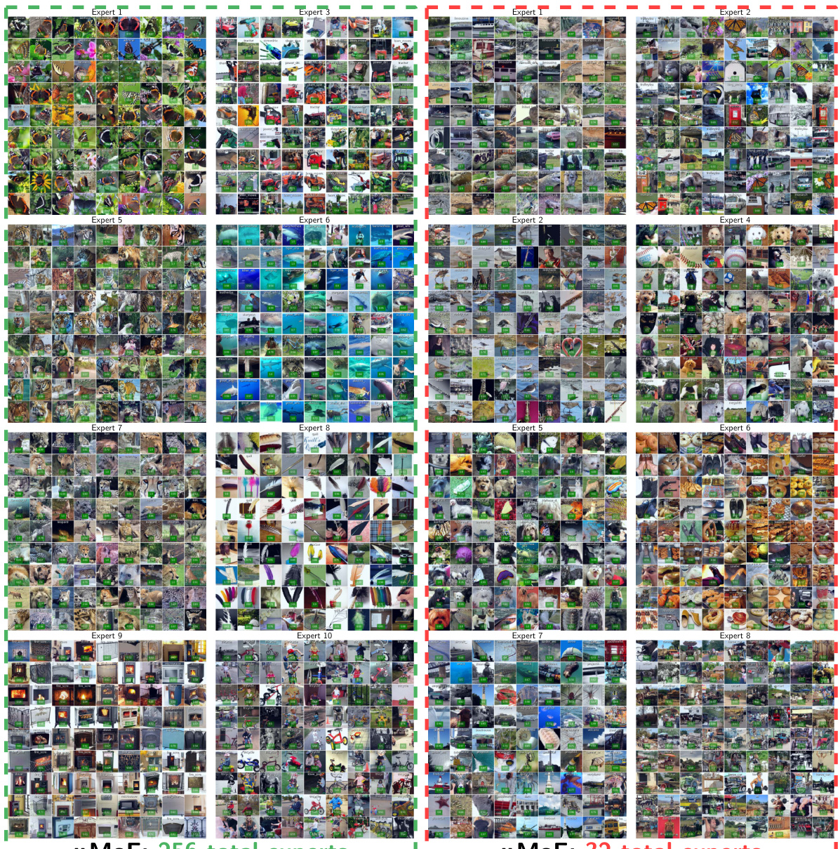
This figure shows a comparison of expert specialization in models with different numbers of experts. The left side shows a model with 256 experts, and the right side shows a model with 32 experts. Each image shows a randomly selected training image that is highly weighted (coefficient ≥ 0.5) by one of the first 10 experts. The figure demonstrates the increased specialization of the experts with a higher number of experts. With more experts, each tends to focus on images within a more narrow semantic range.
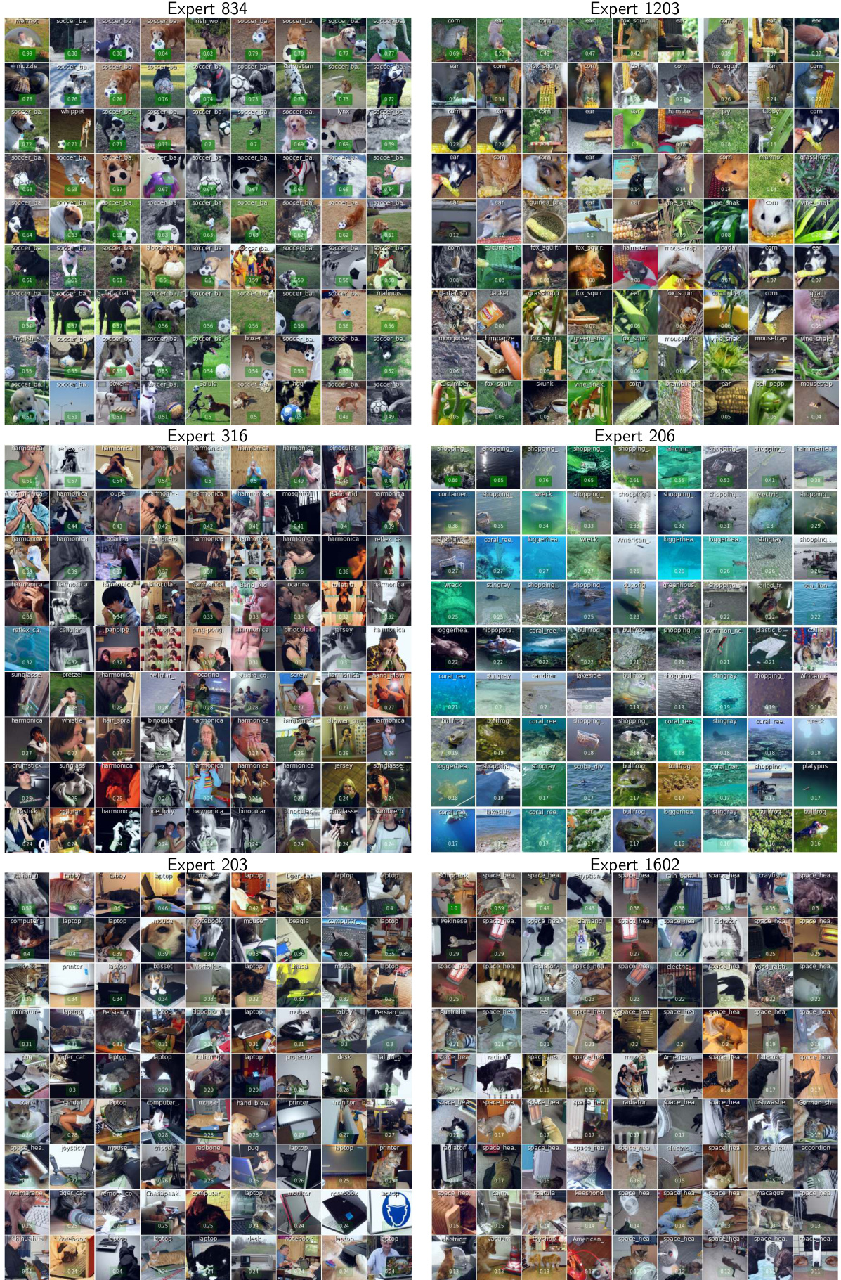
This figure compares the expert specialization in two CPµMoE models fine-tuned on CLIP ViT-B-32 with different numbers of experts (256 and 32). Each row shows a subset of images that strongly activate a particular expert (coefficient ≥ 0.5). The images in each row share visual themes or belong to similar categories. The figure demonstrates that increasing the number of experts leads to greater specialization, with each expert focusing on a more specific set of visual concepts.

This figure compares the qualitative results of using different numbers of experts in CPµMoE layers. The left panel shows results with 256 experts, while the right panel shows results with 32 experts. For each expert, a set of images that have an expert coefficient of at least 0.5 is shown. The figure aims to demonstrate that increasing the number of experts leads to more specialized experts, each focusing on a more specific subset of image categories or visual themes.
This figure compares the qualitative results of using CPµMoE layers with different numbers of experts (256 vs 32). It shows randomly selected images processed by the first ten experts, where the expert coefficient is greater than or equal to 0.5. The images are overlaid with their class labels and expert coefficients. The figure demonstrates that with more experts (256), the experts tend to specialize in processing images from a narrower range of semantic categories, leading to more distinct and specialized subcomputations. With fewer experts (32), each expert is more likely to be involved in processing images from a wider range of categories, resulting in less specialization.

This figure shows the results of an ablation study comparing the use of the softmax and entmax activation functions in CPµMoE-r512 final layers trained on the ImageNet dataset. The x-axis represents the total number of experts used in the CPµMoE layer (on a logarithmic scale), while the y-axis represents the mean expert polysemanticity. The plot shows that for larger numbers of experts, the entmax activation function leads to more specialized experts (lower polysemanticity) compared to softmax. Separate lines are shown for models using DINO and CLIP backbones. The results suggest that entmax is a better choice for achieving increased expert specialisation when using a larger number of experts.
This figure compares the performance of two activation functions, softmax and entmax, in a CPµMoE layer when fine-tuned on ImageNet. The x-axis represents the number of experts used in the CPµMoE layer, while the y-axis shows the mean expert polysemanticity. The plot demonstrates that for a larger number of experts, the entmax activation function leads to experts that are more specialized (monosemantic) compared to the softmax function.

This figure shows the number of training images processed by each expert in the CPµMoE model fine-tuned on the ImageNet1k dataset. Each bar represents an expert, and its height corresponds to the number of images with an expert coefficient of at least 0.5. The x-axis represents the expert index, and the y-axis shows the count of images. The bars are colored to visually differentiate between the experts. The purpose of this visualization is to examine the load distribution among experts, and to verify if some experts are overloaded while others are underutilized.
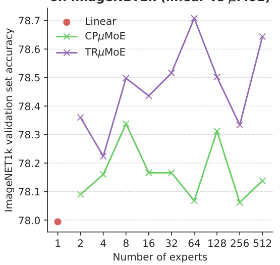
This figure shows the results of fine-tuning the CLIP ViT-B-32 model on the ImageNet1k dataset using different configurations of μMoE layers. The left subplot (a) compares the validation accuracy of using μMoE layers versus linear layers, showing that μMoE layers achieve higher accuracy with the same number of parameters. The right subplot (b) compares the resulting matrix rank for CPμMoE and TRμMoE layers for various expert counts. This demonstrates that TRμMoE offers greater efficiency in parameter usage for a larger number of experts.

This figure shows a comparison of fine-tuning the CLIP ViT-B-32 model on ImageNet using different configurations of μMoE layers. The left subplot (a) compares the validation accuracy achieved with μMoE layers against linear layers, showing that μMoE layers consistently outperform linear layers across various expert counts. The right subplot (b) compares the resulting matrix rank of CPμMoE and TRμMoE layers, illustrating the impact of different factorization choices on model complexity. Both subplots demonstrate that μMoE layers offer competitive performance with comparable parameter counts.

This figure presents a comparative analysis of fine-tuning the CLIP ViT-B-32 model using μMoE layers with varying configurations. The left subplot shows a comparison of the validation accuracy achieved with μMoE layers versus a standard linear layer, demonstrating the performance gains obtained with μMoE. The right subplot compares the rank of the weight matrices for CPμMoE and TRμMoE models as the number of experts is increased. This illustrates the computational efficiency and parameter control offered by TRμMoE for a large number of experts.
This figure shows a comparison of expert specialization in two CPµMoE models fine-tuned on the CLIP ViT-B-32 architecture with different numbers of experts (256 and 32). It presents randomly selected images processed by the top experts in each model, highlighting how increasing the expert count leads to more specialized experts focusing on specific visual themes or image categories. The images are shown with their corresponding expert coefficients. In the model with 256 experts, there is clear specialization of the experts towards specific image classes while the model with 32 experts processes images from various classes, indicating less specialization.
This figure compares the qualitative results of fine-tuning CLIP ViT-B-32 with CPµMoE layers having 256 and 32 experts respectively. For each expert, a selection of images with expert coefficients greater than or equal to 0.5 are displayed. The figure demonstrates that increasing the number of experts leads to more specialized experts. In the model with 32 experts, individual experts are more likely to process images from different semantic categories (polysemantic), while the model with 256 experts shows that the experts mostly process images belonging to similar categories or visual themes (monosemantic).
More on tables

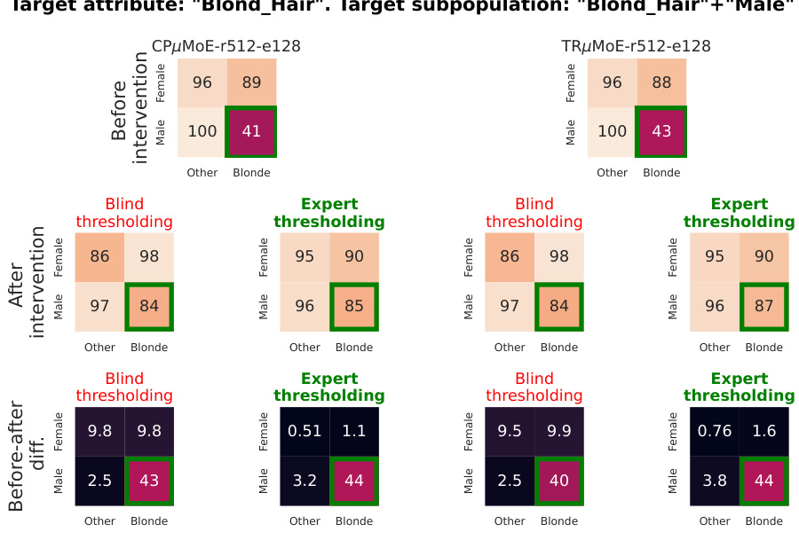
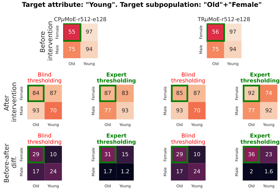
This table shows the fairness metrics for different models and fairness techniques on the CelebA dataset. Two experiments are presented: one targeting bias towards ‘Old females’ for ‘Age’ prediction, and the other targeting bias towards ‘Blond males’ for ‘Blond Hair’ prediction. The metrics used include Equality of opportunity, Standard deviation bias, and Max-Min fairness. The table compares the performance of a linear model, a high-rank linear model, and a CPµMoE model with several fairness techniques, including oversampling, adversarial debiasing, blind thresholding, and the proposed expert thresholding method. The results show the impact of each technique on accuracy and fairness metrics for the target subpopulations.

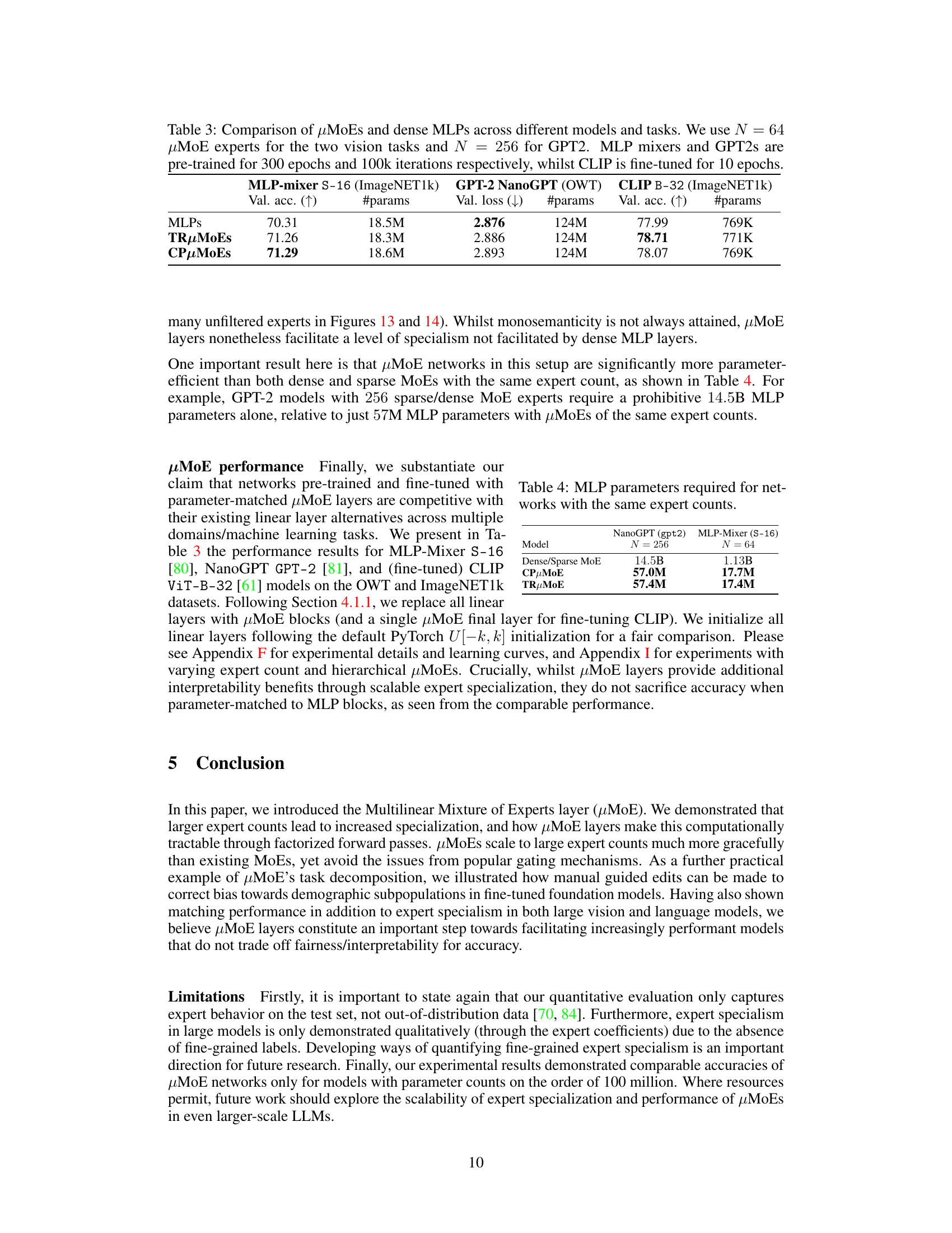
This table compares the performance of models using Multilinear Mixture of Experts (µMoEs) against those using traditional Multilayer Perceptrons (MLPs) across three different tasks: ImageNet1k classification using MLP-Mixer S-16, OpenWebText language modeling using GPT-2 NanoGPT, and ImageNet1k fine-tuning using CLIP B-32. The number of µMoE experts used is 64 for the vision tasks and 256 for the language task. The models were trained for different durations (300 epochs for MLP-Mixers and GPT-2, 10 epochs for CLIP). The table shows the validation accuracy/loss and the number of parameters for each model and task.

This table compares the number of parameters required for Multilayer Perceptron (MLP) networks with the same number of experts, using different Mixture of Experts (MoE) models. It shows that µMoE layers (both CPµMoE and TRµMoE) are significantly more parameter-efficient than dense or sparse MoE layers, especially when dealing with large numbers of experts.

This table compares the proposed Multilinear Mixture of Experts (μMoE) model with existing Mixture of Experts (MoE) models in terms of differentiability, parameter efficiency, and FLOP efficiency. It highlights the advantages of μMoEs, which are differentiable by design and avoid the restrictive parameter and computational costs of dense MoEs while not inheriting the training issues associated with sparse MoEs.

This table compares the computational cost (number of parameters and FLOPs) and the maximum rank of the expert weight matrices for different MoE layer implementations: Dense MoE, Sparse MoE, CPµMoE, and TRµMoE. It shows that CPµMoE and TRµMoE are more parameter-efficient than Dense and Sparse MoEs, especially for a large number of experts (N). The table also indicates that TRµMoE can be more computationally efficient than CPµMoE in terms of FLOPs for larger N.

This table compares the peak memory usage and latency of different layer types: linear layer, dense MoE, sparse MoE, TRμMoE, and CPμMoE. The comparison is made for a single input and uses 128 experts in each MoE layer, with the μMoE ranks matched to the linear layers. The results show the relative resource efficiency of the different approaches, highlighting the advantages of the proposed μMoE layers in terms of both memory usage and latency.

This table summarizes the experimental setup used for training the MLP-mixer, NanoGPT, and CLIP models. It includes hyperparameters such as learning rate, batch size, weight decay, warmup steps, training duration, stochastic depth, RandAugment strength, dropout, mixup strength, mixed precision, random seed, and hardware used.

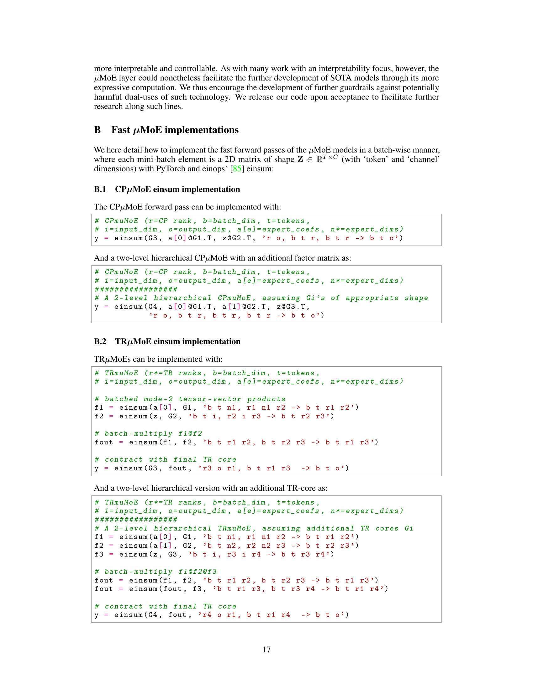
This table compares the computational cost (in FLOPs) of the original µMoE layer implementation with the optimized fast einsum implementation presented in Appendix B. It highlights the significant reduction in computational cost achieved by the optimized approach for a specific configuration with 512 experts and 768-dimensional input/output.

This table shows the ImageNet1k validation accuracy of hierarchical MLP-mixer models with different numbers of experts per block after 300 epochs of pre-training. It compares the performance of standard MLPs against both CPµMoE and TRµMoE models with different levels of hierarchy (1 and 2 levels). The number of parameters for each model is also provided.

This table shows the results of fine-tuning a CLIP ViT-B-32 model on ImageNet1k using hierarchical μMoEs with varying numbers of experts and levels of hierarchy. It compares the validation accuracy, number of parameters, and parameter counts for different model configurations (hierarchical CPμMoEs and TRμMoEs) against a baseline model with a single linear layer. The table highlights the parameter efficiency of hierarchical μMoEs, especially when compared to regular MoEs.

This table shows the impact of using hierarchical μMoE layers (with different numbers of hierarchy levels) on the validation accuracy of a CLIP ViT-B-32 model fine-tuned on ImageNet1k. It compares the performance against a single-level μMoE and a regular MoE. The table also details the number of parameters used for each model and configuration.
Full paper#


