↗ OpenReview ↗ NeurIPS Homepage ↗ Chat
TL;DR#
Causal discovery from time series data is crucial across many scientific domains, yet challenging. Traditional methods like Granger causality often fail in complex, interacting systems. Convergent Cross Mapping (CCM) was proposed as an alternative, focusing on the topological properties of dynamical systems, but often yields inaccurate results depending on data quality.
The proposed Tangent Space Causal Inference (TSCI) method directly addresses this issue. TSCI uses vector fields as explicit representations of system dynamics, checking synchronization between them to detect causalities. It’s model-agnostic, more effective than basic CCM with minimal extra computation, and can be enhanced with latent variable models or deep learning. Experiments on benchmark systems demonstrated improved performance.
Key Takeaways#
Why does it matter?#
This paper is important because it introduces a novel method, Tangent Space Causal Inference (TSCI), for causal discovery in dynamical systems. This addresses limitations of existing methods like Convergent Cross Mapping (CCM) by leveraging vector fields and improving accuracy and interpretability. TSCI’s model-agnostic nature and potential for integration with deep learning make it a significant contribution to causal inference research. This opens avenues for further exploration in various fields that rely on time-series analysis.
Visual Insights#
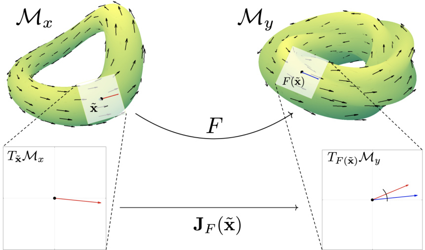
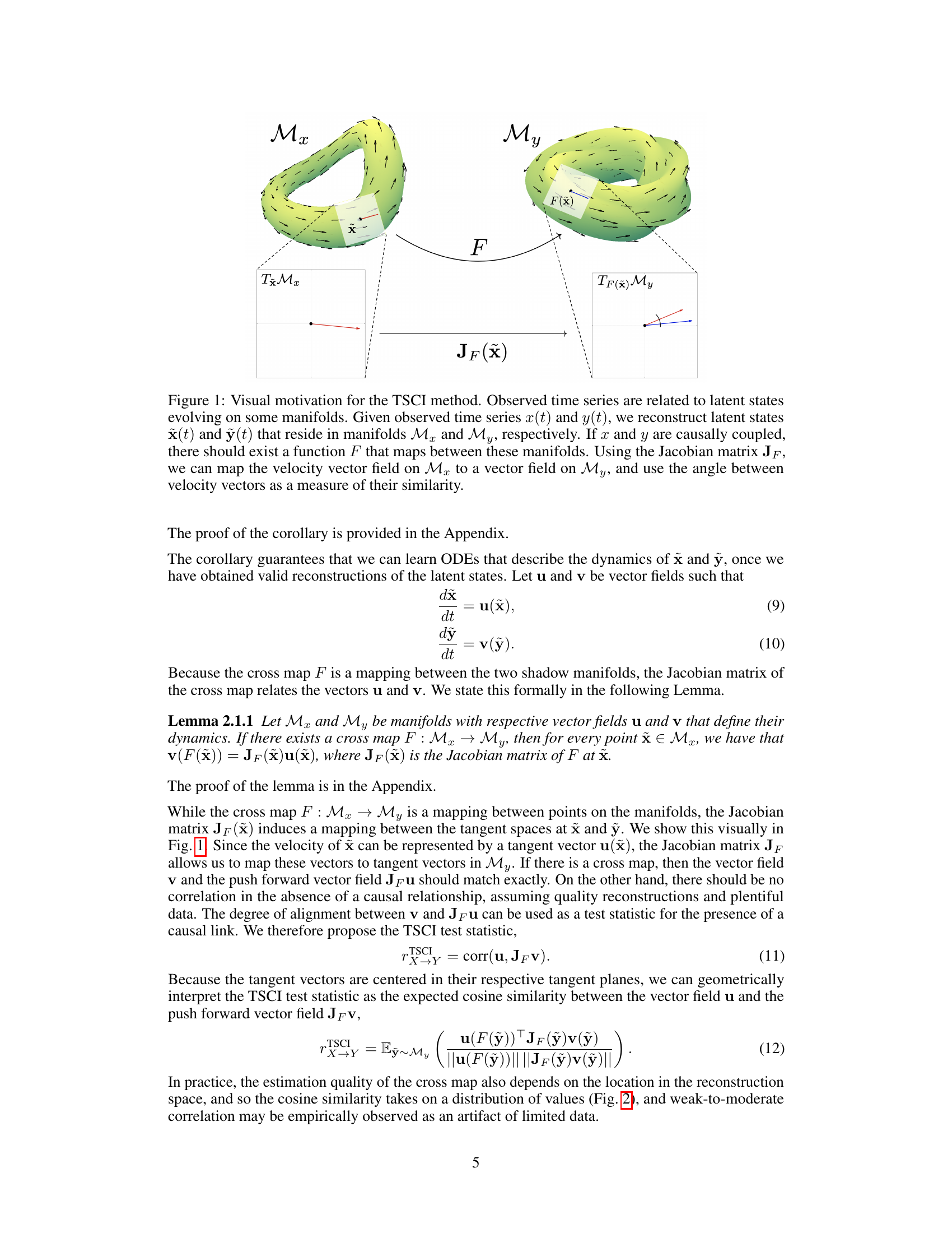
This figure provides a visual explanation of the Tangent Space Causal Inference (TSCI) method. It shows two manifolds, Mx and My, representing the latent state spaces of two observed time series, x(t) and y(t). A function F maps between these manifolds, and its Jacobian matrix, JF(x), transforms tangent vectors from the tangent space of Mx (TxMx) to the tangent space of My at F(x) (TF(x)My). The angle between the transformed and original tangent vectors provides a measure of similarity, which is used by TSCI to infer causality.
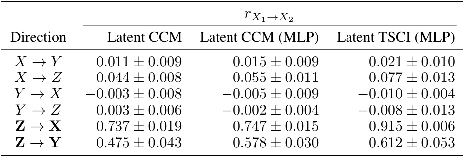
This table presents the results of causal inference experiments on a double pendulum system. The experiment used latent CCM (with and without MLPs) and latent TSCI (with MLPs) to infer causal relationships between different parts of the system (X1, X2, Y, Z). The table shows the mean and standard deviation of the test statistic (correlation coefficient) for each inferred causal direction, allowing comparison between methods and highlighting the accuracy of each in identifying the true causal relationships.
In-depth insights#
Tangent Space CI#
The heading ‘Tangent Space Causal Inference’ suggests a novel approach to causal discovery in dynamical systems. It likely builds upon existing methods like Convergent Cross Mapping (CCM), addressing their limitations by leveraging the geometry of the systems’ state spaces. Instead of directly comparing time series, this approach probably focuses on the vector fields representing the systems’ dynamics. This could lead to more robust causal inference, especially in high-dimensional or noisy systems where traditional methods struggle. The use of tangent spaces, which are spaces approximating local changes in the manifold, implies a focus on local dynamics rather than global patterns, improving the accuracy and potentially reducing the sensitivity to the choice of embedding parameters. By utilizing tangent spaces, the method is likely more robust to noise and distortions in the data. The ‘Tangent Space CI’ is likely to outperform CCM in detecting causal relationships, providing a principled alternative to CCM with improved interpretability. The method might still suffer from limitations concerning high-dimensional data and complex system dynamics, which need to be addressed in future research.
CCM Enhancement#
Convergent Cross Mapping (CCM) enhancements are crucial for reliable causal inference in complex systems. Improving the accuracy of cross-map construction is paramount, as inaccuracies lead to spurious causal relationships. This can involve better methods for embedding the time series data into a state space, handling noisy data more effectively, and addressing the limitations of relying on nearest-neighbor techniques. Incorporating advanced machine learning techniques, such as neural networks or Gaussian processes, allows for more flexible and robust cross-map estimation. Addressing issues like short time series and the challenge of distinguishing true causality from indirect influences require more sophisticated methods, potentially by exploiting information theoretical measures or leveraging latent variable models. The development of more interpretable test statistics and methodologies for assessing statistical significance is also vital for more reliable interpretation of CCM results. Ultimately, CCM enhancement efforts aim to make it a more powerful and trustworthy tool for analyzing causal relationships in diverse dynamic systems.
Model Agnostic TSCI#
The concept of ‘Model Agnostic TSCI’ suggests a significant advancement in causal inference within dynamical systems. Its model-agnostic nature is a strength, allowing flexibility in choosing the method for learning the cross-map function (e.g., MLPs, splines, Gaussian processes). This adaptability is crucial because the optimal method can vary depending on the specific characteristics of the data and the underlying system. Unlike traditional methods that are tightly coupled to specific model assumptions, TSCI’s flexibility improves robustness and generalizability. Furthermore, TSCI’s reliance on explicit representation of system dynamics through vector fields offers a more nuanced and arguably more accurate approach to causal discovery compared to methods solely relying on correlation-based metrics. This approach provides a potentially more robust and interpretable alternative to existing techniques, while retaining the efficiency of related methods. The focus on tangent space analysis is particularly powerful in leveraging geometric properties for accurate causal directionality determination. However, further research should explore the sensitivity of TSCI to noise and sparsity in time series data and the development of robust methods for estimating vector fields in complex systems.
Benchmark Systems#
The selection of benchmark systems for evaluating causal inference methods is crucial. Ideal benchmarks should exhibit known causal relationships with varying complexities, allowing for a nuanced assessment of algorithm performance. Diverse system types are needed, encompassing linear and nonlinear dynamics, to check for robustness. Control over parameters such as coupling strength or noise levels would facilitate systematic evaluation across different conditions. Inclusion of both simple and high-dimensional systems is important, reflecting real-world data complexities. Finally, using established benchmarks (like those in the paper’s references) enables comparison to existing results and fosters community-wide progress in causal discovery. The thoroughness of this evaluation directly impacts the reliability and trustworthiness of any proposed method.
Future Directions#
Future research could explore more sophisticated methods for estimating vector fields from time series data, potentially leveraging deep learning or other advanced techniques to enhance accuracy and robustness in noisy or incomplete datasets. Investigating the performance of TSCI across a wider variety of dynamical systems is crucial, particularly focusing on systems with complex interactions, high dimensionality, or non-stationarity. The impact of different embedding methods and parameter choices on TSCI’s accuracy and efficiency requires further study. A comparative analysis of TSCI against other causal inference methods on real-world datasets, highlighting its strengths and limitations in various application domains, would be beneficial. Finally, exploring extensions of TSCI to handle multivariate time series data and incorporating latent variable models to disentangle complex causal relationships would unlock its potential in a broader range of scenarios.
More visual insights#
More on figures
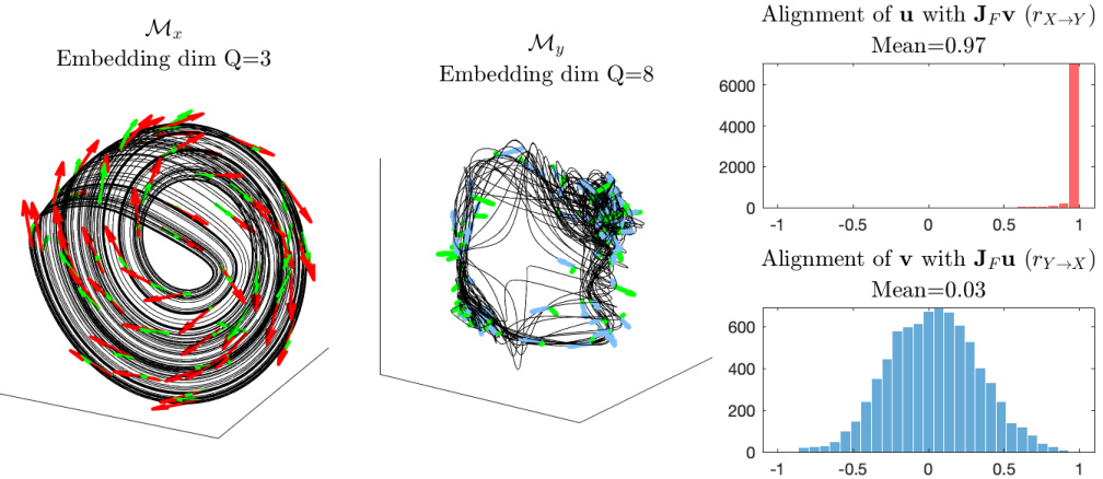
This figure visualizes the shadow manifolds (Mx and My) of a unidirectionally coupled Rössler-Lorenz system (with coupling strength C=1). It shows the manifolds with tangent vectors overlaid, illustrating the concept of mapping vector fields between manifolds using Jacobian matrices. The histograms display the distribution of cosine similarities between the tangent vectors of one manifold and the mapped tangent vectors from the other manifold, for both directions (x→y and y→x). The means of these distributions represent the TSCI test statistics, which reveal the degree of similarity between the vector fields and, therefore, the causal relationship between the systems.
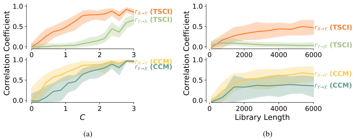
This figure compares the performance of Tangent Space Causal Inference (TSCI) and Convergent Cross Mapping (CCM) methods on a unidirectionally coupled Rössler-Lorenz system. Subfigure (a) shows how the median test statistic of both methods varies with the coupling strength (C) between the two systems, while subfigure (b) demonstrates the impact of library length (the length of the time series used for analysis) on the test statistic for a fixed coupling strength of C=1.0. Shaded areas represent the 5th and 95th percentiles across 100 trials, illustrating variability in performance.

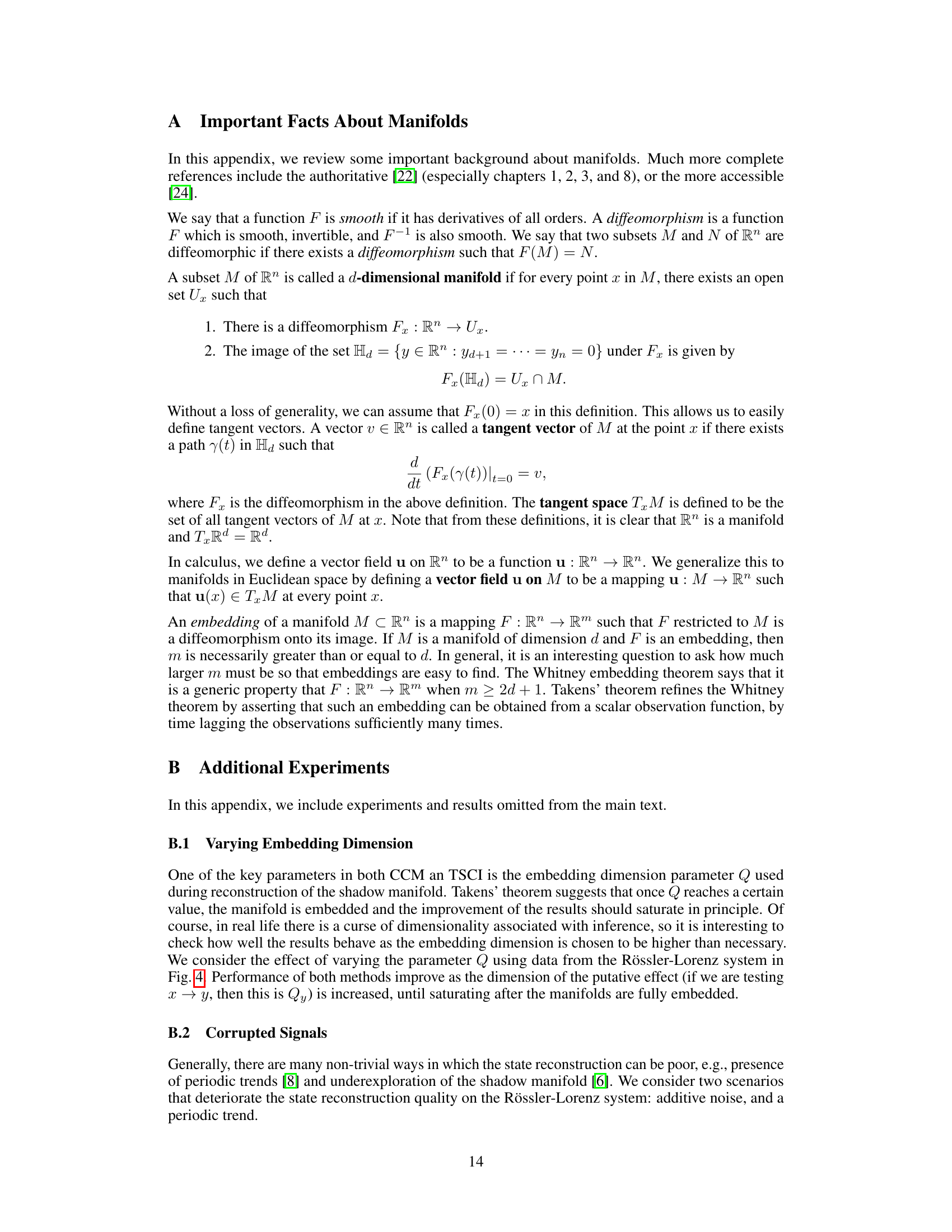
This figure compares the performance of Tangent Space Causal Inference (TSCI) and Convergent Cross Mapping (CCM) methods in detecting causal relationships in a unidirectionally coupled Rössler-Lorenz system. The heatmaps illustrate the test statistics (correlation coefficients) for different embedding dimensions (Qx and Qy) for both methods, showing the direction of causality (X→Y or Y→X). The red lines represent the embedding dimensions selected by a false-nearest neighbor algorithm which helps determine the optimal number of dimensions to accurately capture the system’s dynamics. The figure aims to demonstrate that TSCI is more robust in detecting the true causality compared to CCM across various embedding dimensions.
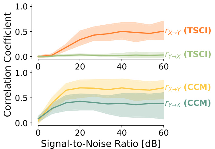
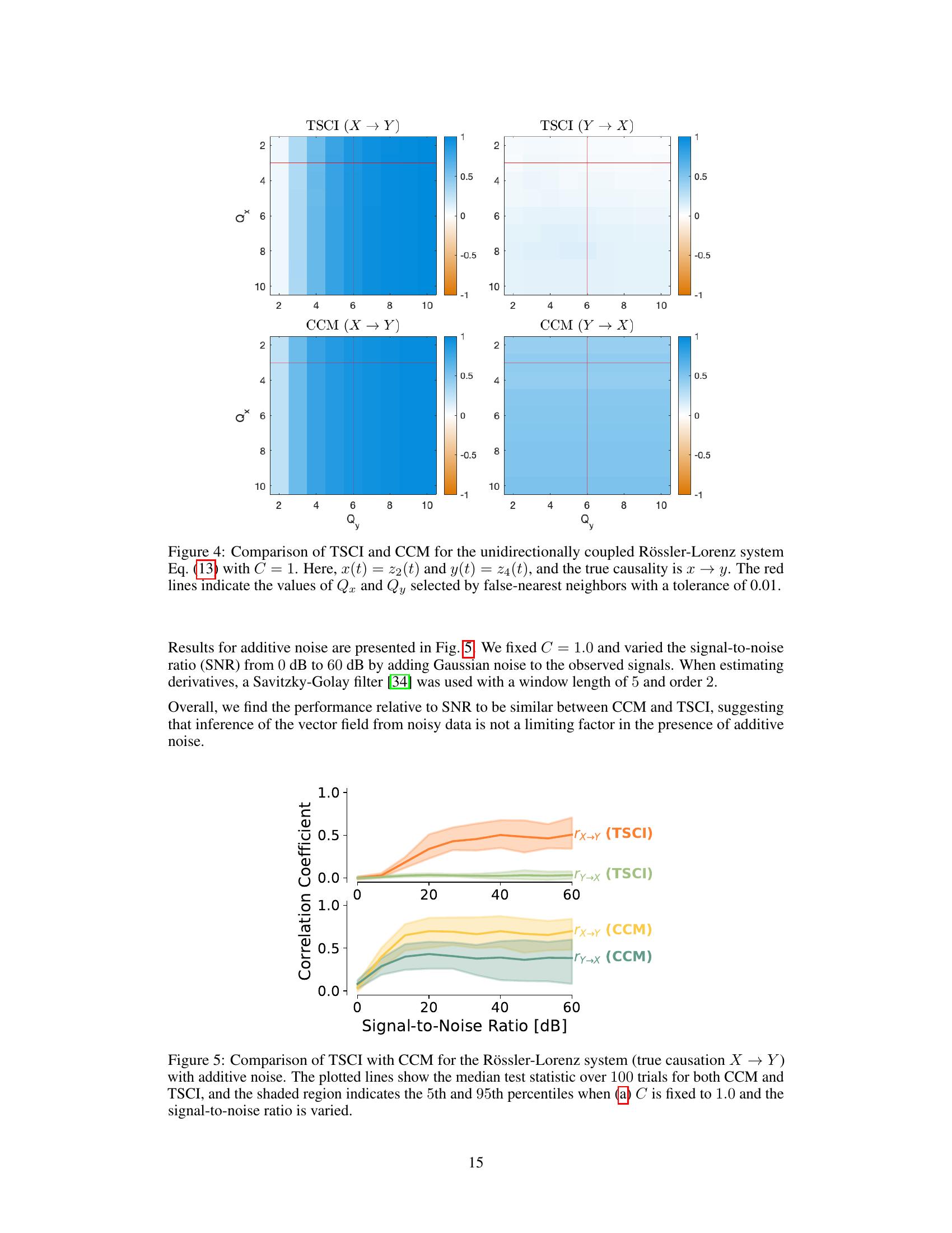
The figure compares the performance of TSCI and CCM in the presence of additive noise in the Rössler-Lorenz system. It shows the median test statistic and its 5th and 95th percentiles over 100 trials for both algorithms, while varying the signal-to-noise ratio. The true causal relationship is X → Y. The shaded areas represent the variability of the results.

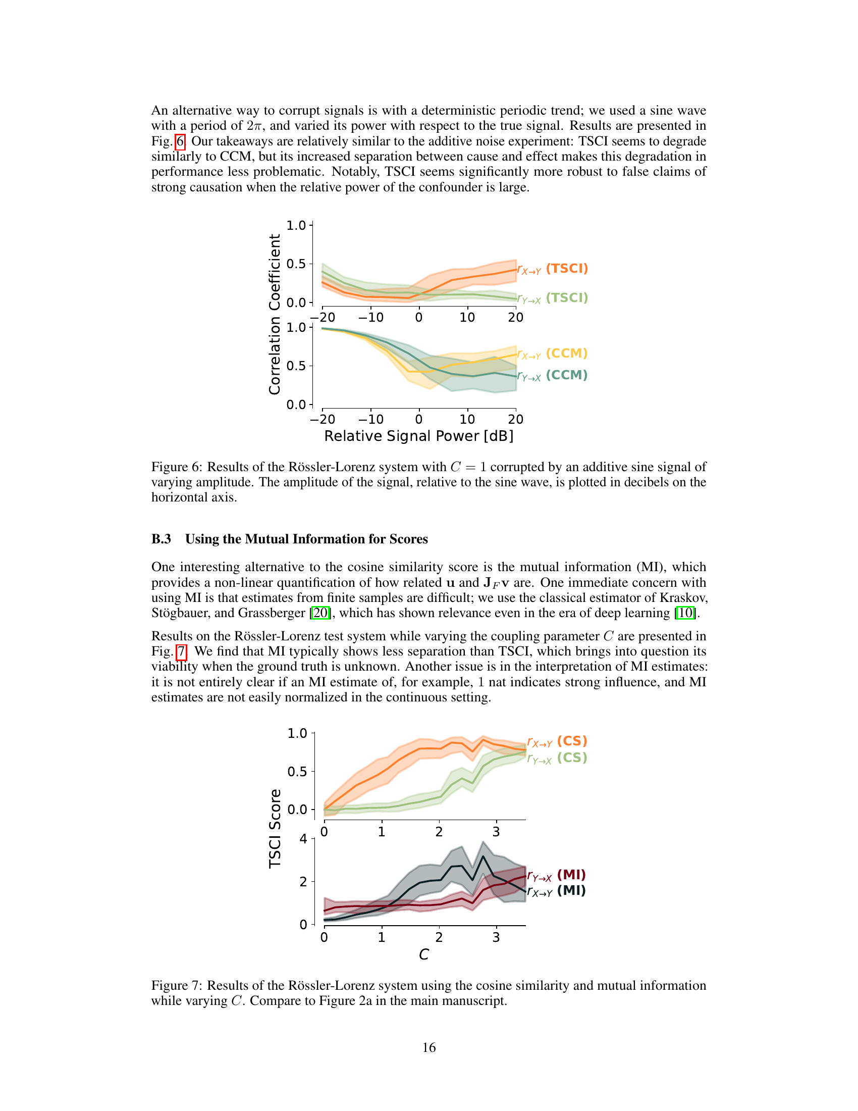
This figure compares the performance of TSCI and CCM in detecting causality when the Rössler-Lorenz system is affected by an additive sine wave signal. The x-axis represents the relative signal power of the sine wave in dB, which is varied to simulate different levels of signal corruption. The y-axis shows the correlation coefficient, a measure of the strength of the detected causal relationship. The plot displays the median test statistic over 100 trials, with shaded regions showing the 5th and 95th percentiles. Separate lines are plotted for both the true causal direction (x→y) and the opposite direction (y→x) for both TSCI and CCM. The results show that both methods’ performance degrades as the sine wave’s relative power increases, meaning that higher signal corruption negatively impacts the accuracy of causal inference. However, TSCI shows greater resilience to false claims of strong causation at higher relative signal powers than CCM.

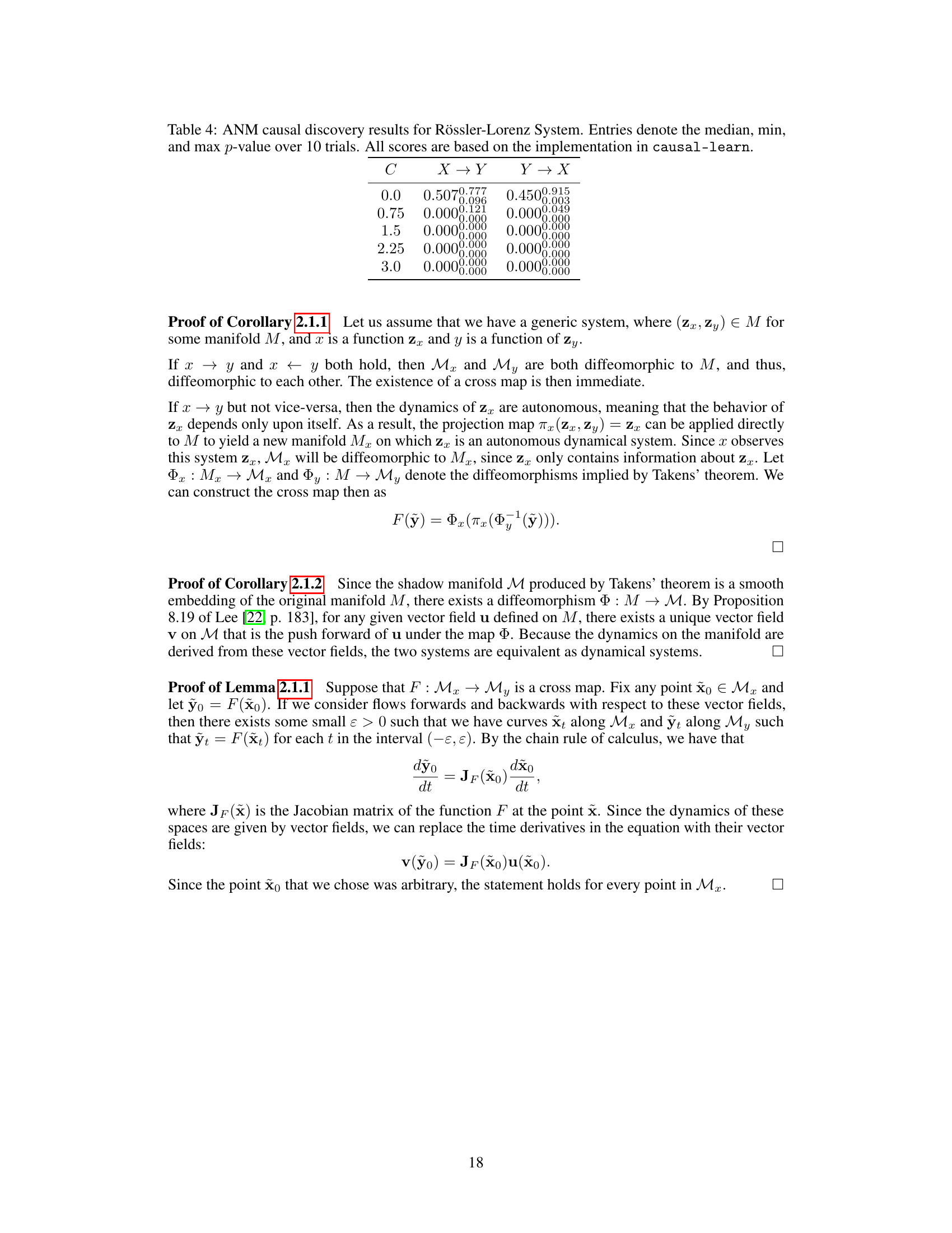
This figure compares the results obtained using cosine similarity (CS) and mutual information (MI) as test statistics for the TSCI algorithm applied to a Rössler-Lorenz system with varying coupling strength (C). The top panel displays the results using cosine similarity, while the bottom panel shows the results using mutual information. Each panel shows the TSCI scores (rx→y and ry→x) for both the causal direction (x → y) and the reversed direction (y → x) as a function of C. The shaded areas represent confidence intervals, highlighting the variability of the results. This figure serves to compare the performance and interpretability of cosine similarity against mutual information as test statistics in the TSCI approach.
More on tables

This table presents the results of Granger causality tests performed on the Rössler-Lorenz system for various coupling strengths (C). It shows the median, 5th, and 95th percentile p-values from the F-test for both directions of causality (X → Y and Y → X) across 50 trials. The p-values indicate the statistical significance of the causal relationship between the two systems. Lower p-values suggest stronger evidence of a causal relationship.

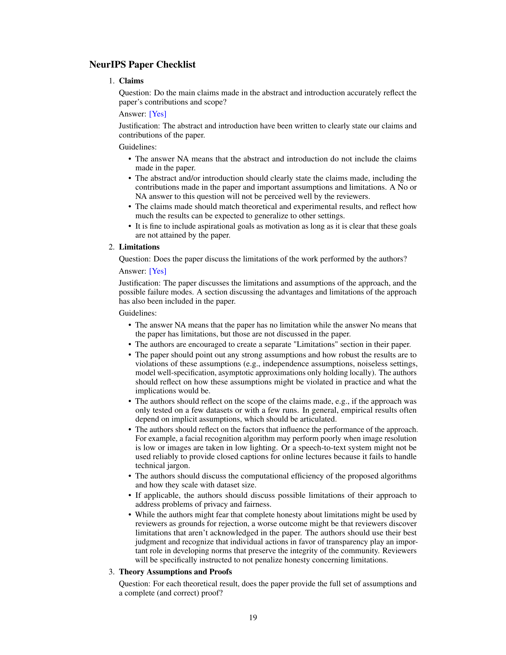
This table presents the results of three bivariate causal discovery methods (RECI, IGCI, and ANM) applied to the Rössler-Lorenz system with varying coupling strengths (C). A negative score indicates causality from X to Y, and a positive score indicates causality from Y to X. The median, minimum, and maximum scores across ten trials are shown for each method and coupling strength.

This table presents the results of Granger causality tests performed on the Rössler-Lorenz system for various coupling strengths (C). The p-values indicate the strength of evidence for causality in both directions (X→Y and Y→X). Lower p-values suggest stronger evidence for causality.
Full paper#

