↗ OpenReview ↗ NeurIPS Homepage ↗ Chat
TL;DR#
Estimating treatment effects over time is crucial in many fields, but existing methods struggle with time-varying confounders, selection bias, and long-term dependencies, especially when making long-term predictions. Many existing methods have also disregarded the importance of invertible representation in counterfactual analysis, compromising identification assumptions. These issues make it difficult to accurately estimate how different treatment plans would impact individual outcomes over time.
The paper introduces Causal CPC, a new approach to counterfactual regression over time that addresses these issues. By using recurrent neural networks (RNNs) combined with Contrastive Predictive Coding (CPC) and Information Maximization (InfoMax), Causal CPC effectively captures long-term temporal dynamics and ensures identification assumptions are met. Experimental results demonstrate state-of-the-art performance on both synthetic and real-world datasets. The method is also computationally efficient, making it practical for real-world applications.
Key Takeaways#
Why does it matter?#
This paper is crucial for researchers working on causal inference and time-series analysis, especially in applications like personalized medicine and policy evaluation. It offers a novel and efficient approach to counterfactual regression, combining RNNs, CPC, and InfoMax, achieving state-of-the-art results. This work opens new avenues for research, including applying contrastive learning to causal problems and developing uncertainty-aware models for longitudinal data.
Visual Insights#
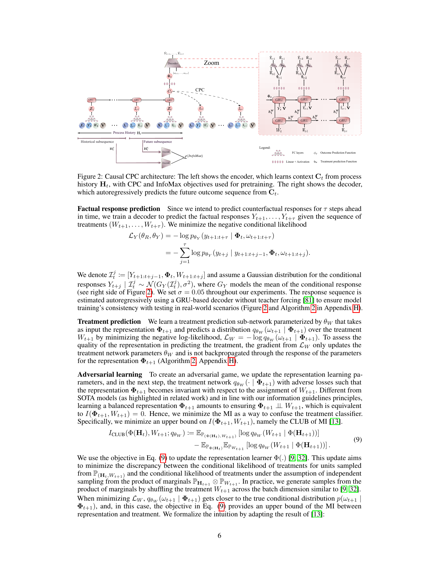
The figure illustrates the architecture of the Causal CPC model. The left side shows the encoder, which takes the process history Ht as input and generates a context representation Ct using a GRU and contrastive predictive coding (CPC). The InfoMax principle is also applied to improve the representation’s invertibility. The right side shows the decoder, which takes Ct and autoregressively predicts future outcome sequences. The figure also highlights how the model handles both short-term and long-term dependencies.

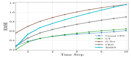
This table presents the RMSEs (Root Mean Squared Errors) for the semi-synthetic MIMIC III dataset with a sequence length of 100. The results are shown for different prediction horizons (τ = 1 to τ = 10) and different models: Causal CPC (the proposed model), CT (Causal Transformer), G-Net, CRN (Counterfactual Recurrent Networks), and RMSN (Recurrent Marginal Structural Networks). Lower RMSE values indicate better performance. The table shows how the RMSE increases as the prediction horizon increases for all models, but Causal CPC consistently outperforms the other models across all horizons.
In-depth insights#
Causal Contrastive CPC#
The proposed “Causal Contrastive CPC” method presents a novel approach to counterfactual regression over time, particularly focusing on long-term predictions. It cleverly leverages the efficiency of Recurrent Neural Networks (RNNs), eschewing computationally expensive transformers, while incorporating Contrastive Predictive Coding (CPC) to capture long-term dependencies and the InfoMax principle to ensure invertible representations, addressing a weakness in many existing methods. The use of CPC allows the model to learn rich representations of temporal data by contrasting future with past information, enhancing predictive capability. Furthermore, the integration of InfoMax, by maximizing mutual information between input and representation, implicitly enforces invertibility, crucial for valid causal inference. The resulting model demonstrates improved accuracy and efficiency on both synthetic and real-world datasets, showing the potential to improve causal inference in various domains. The adversarial training process to balance representation across treatment regimes is a key innovation, directly tackling the issue of selection bias often encountered in time-series causal inference.
Longitudinal Causal Effects#
Analyzing longitudinal causal effects requires a nuanced understanding of time-dependent confounding, where past events influence future outcomes and treatments. Identifying and addressing such confounding is crucial for obtaining unbiased estimates of causal effects over time. This often involves sophisticated statistical modeling that accounts for the temporal nature of the data, such as marginal structural models (MSMs) or more modern techniques like recurrent neural networks (RNNs). Invertibility of representation is also important as it ensures that identification assumptions used in causal inference methods are valid in the representation space. Failure to achieve this can lead to biased estimates. The use of techniques such as contrastive predictive coding (CPC) and Information Maximization (InfoMax) shows promise in capturing long-term temporal dependencies and building better representations, which are key for accurate and efficient causal inference. These methods often involve self-supervised learning, which helps to learn robust representations that are less susceptible to spurious associations.
RNNs for Time Series#
Recurrent Neural Networks (RNNs), particularly LSTMs and GRUs, are powerful tools for time series analysis due to their inherent ability to handle sequential data. Their recurrent architecture allows information from previous time steps to influence the prediction at the current step, capturing temporal dependencies crucial for accurate forecasting. This makes RNNs well-suited for tasks like time series forecasting, anomaly detection, and classification. However, vanilla RNNs suffer from vanishing and exploding gradients, which limit their ability to learn long-range dependencies. LSTMs and GRUs mitigate this problem through sophisticated gating mechanisms, enabling them to capture more intricate temporal patterns over extended periods. Despite these advantages, RNNs can be computationally expensive, particularly when dealing with long sequences. Furthermore, training RNNs can be challenging and requires careful hyperparameter tuning to prevent overfitting and ensure convergence. Therefore, advancements in attention mechanisms and transformer networks offer alternative approaches for certain time series tasks, potentially providing greater efficiency and scalability.
InfoMax for Invertibility#
The concept of ‘InfoMax for Invertibility’ in the context of a time-series causal inference model is a crucial innovation. It directly addresses a critical weakness in many existing approaches: the lack of invertibility in the learned representations. Non-invertible representations can compromise identification assumptions, making it difficult to reliably estimate counterfactual outcomes. By maximizing mutual information (MI) between the input (process history) and its representation, InfoMax encourages the learned representation to be highly informative about the original process. This implicitly promotes invertibility, as it implies that the original history can be reasonably reconstructed from the representation. This is especially valuable when dealing with time-varying confounders, where ensuring the representation maintains sufficient information about the historical context is vital for accurate causal inference. The use of InfoMax also offers a computationally efficient alternative to using explicit decoders for representation invertibility, which are known to add significant complexity to models. This makes the approach particularly appealing when dealing with the high-dimensional data often encountered in real-world time-series problems. The theoretical grounding of InfoMax for representation invertibility helps strengthen the validity of counterfactual estimations, which is a major contribution to the field of causal inference.
Ablation Study & Limits#
An ablation study systematically removes components of a model to assess their individual contributions. In the context of a counterfactual regression model, this might involve removing or disabling specific regularization terms (like InfoMax or contrastive loss), architectural elements (like the GRU layers), or even the contrastive predictive coding (CPC) mechanism entirely. The results would quantify the impact of each component on model performance, potentially highlighting critical aspects necessary for achieving state-of-the-art results. Understanding these individual contributions helps to clarify the model’s inner workings and pinpoint strengths and weaknesses. The limits section of such a study would discuss inherent constraints. For example, the model’s performance may degrade when assumptions like sequential ignorability are violated or when faced with high levels of confounding or data sparsity. The limitations section also analyzes inherent challenges in counterfactual inference related to long-term predictions and potential biases caused by unobserved confounders or model design choices. By carefully considering both the ablation findings and the inherent limits, researchers can better understand the model’s capabilities, applicability, and areas needing further development or improvement.
More visual insights#
More on figures

The figure illustrates the Causal CPC architecture, showing both encoder and decoder components. The encoder uses GRUs and contrastive predictive coding (CPC) to learn a context representation Ct from the process history Ht. This process also includes InfoMax regularization to make the representation invertible. The decoder then uses the context representation Ct to autoregressively predict the future outcome sequence.

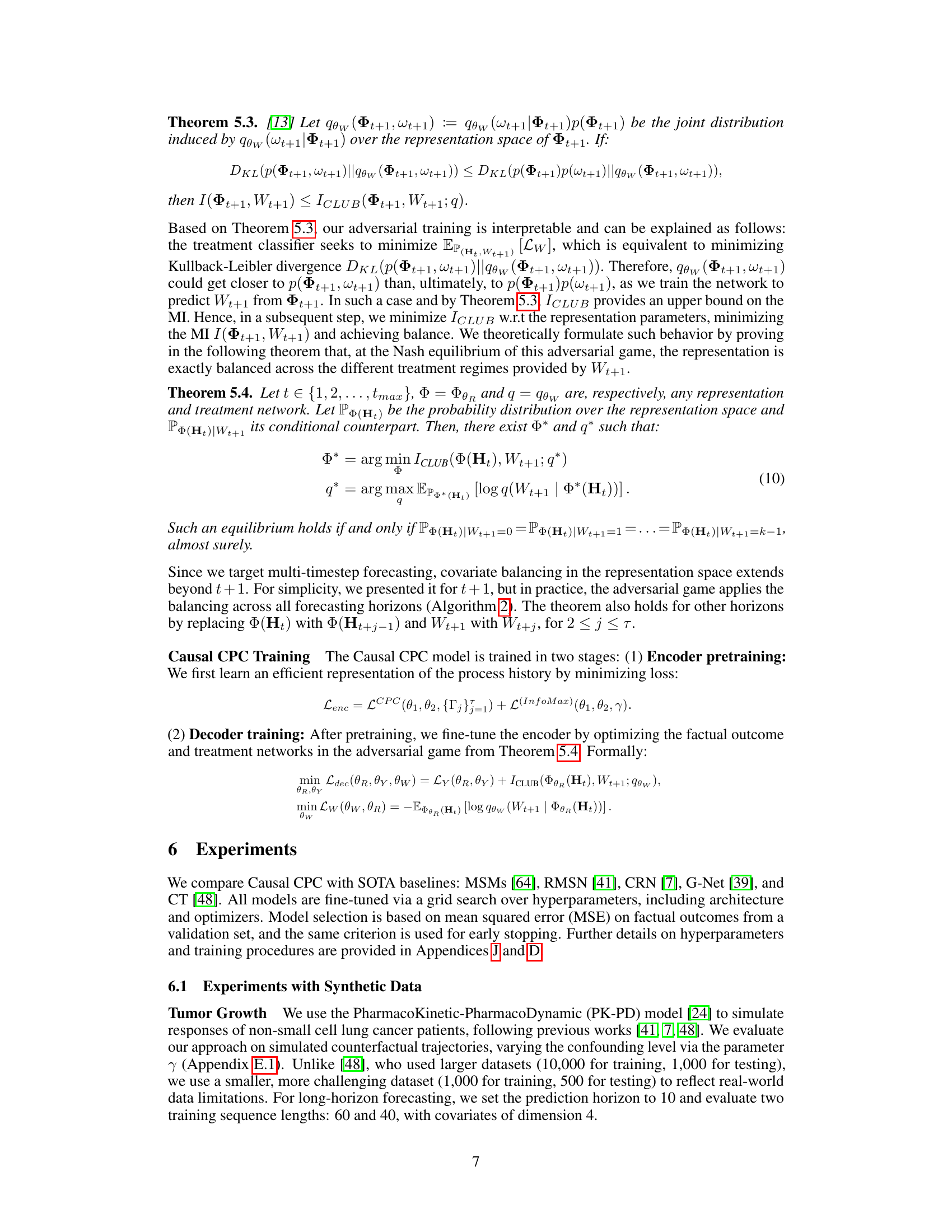
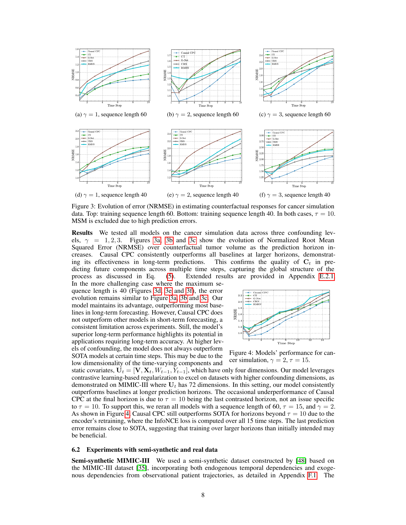
This figure displays the performance of different models in predicting counterfactual tumor volume over time for a cancer simulation dataset. The normalized root mean squared error (NRMSE) is plotted against the time step for each model. Two sets of results are shown, one for a training sequence length of 60 and another for a length of 40. In both cases, the prediction horizon (τ) is set to 10. The Marginal Structural Model (MSM) is excluded because of its high prediction errors. The figure helps to visualize how well each model can predict counterfactual outcomes, especially over longer time horizons and with different training sequence lengths. It illustrates the superiority of Causal CPC, especially for longer prediction horizons.
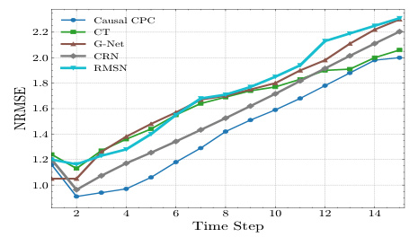
This figure shows the performance of Causal CPC and several other models in estimating counterfactual tumor volumes in a cancer simulation. The normalized root mean squared error (NRMSE) is plotted against the time step for different prediction horizons (τ = 1, 2, 3). Two sets of results are presented: one where the training sequence length was 60 days and another where it was 40 days. The results highlight the superior performance of Causal CPC at longer time horizons (larger τ). MSM was excluded because its prediction errors were too large to be meaningfully included in the plots.
This figure displays the evolution of the Normalized Root Mean Squared Error (NRMSE) over time steps for the task of estimating counterfactual tumor volumes in a cancer simulation. The results are shown for three different levels of confounding (γ = 1, 2, 3) and two different training sequence lengths (60 and 40). The figure highlights the superior performance of the proposed Causal CPC method compared to other methods, especially at longer prediction horizons (time steps). The Marginal Structural Model (MSM) is excluded because it showed excessively high prediction errors.

This figure displays the evolution of the Normalized Root Mean Squared Error (NRMSE) across different prediction horizons (time steps) for counterfactual tumor volume estimation using various models. The results are shown for two training sequence lengths (60 and 40) and three levels of confounding (γ = 1, 2, 3). The figure highlights the performance of Causal CPC in comparison to other state-of-the-art baselines. It demonstrates that Causal CPC consistently outperforms the other methods as the prediction horizon increases, especially when the training sequence length is longer and the confounding level is higher. This suggests the method’s effectiveness for long-term counterfactual regression. The MSM model is excluded from the figure due to significantly high prediction errors.
The figure shows the performance of Causal CPC and other models in estimating counterfactual tumor volumes over time, using the cancer simulation data. It presents the Normalized Root Mean Squared Error (NRMSE) against the prediction horizon (time steps). The top row displays results for training sequences of length 60, while the bottom row shows results for sequences of length 40. In both cases, the prediction horizon (τ) is set to 10. The Marginal Structural Model (MSM) is excluded because its prediction errors were too high to be meaningfully plotted.

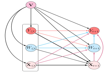
This figure shows a causal graph that illustrates the relationships between different variables in the model. The variables include static confounders (V), time-varying contexts (X), treatments (W), and outcomes (Y), all observed up to a given time t. The figure illustrates the impact of past treatments and covariates on future treatments and outcomes, and highlights the process history Ht+1, which is a summary of all variables up to time t+1. This history is used as input for the causal inference task.
More on tables

This table presents a comparison of the model complexity (in terms of the number of trainable parameters) and computational efficiency (training and prediction times) across different models. The results are based on the tumor growth simulation dataset with a confounding level of γ = 1, using a single NVIDIA Tesla M60 GPU for training. The table shows that Causal CPC demonstrates a good balance between accuracy and computational efficiency.

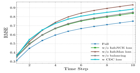
This table presents the results of an ablation study conducted to evaluate the impact of different components of the proposed Causal CPC model. The study measures the Normalized Root Mean Squared Error (NRMSE) for prediction horizons from 1 to 10, across two datasets: a cancer simulation dataset and a semi-synthetic MIMIC III dataset. By removing different parts of the model, such as the InfoNCE loss, the InfoMax loss, the balancing mechanism, or replacing the ICLUB objective with the CDC loss, the study aims to understand the contributions of each component to the overall model performance. The results show that removing any of the key components reduces the model’s accuracy.

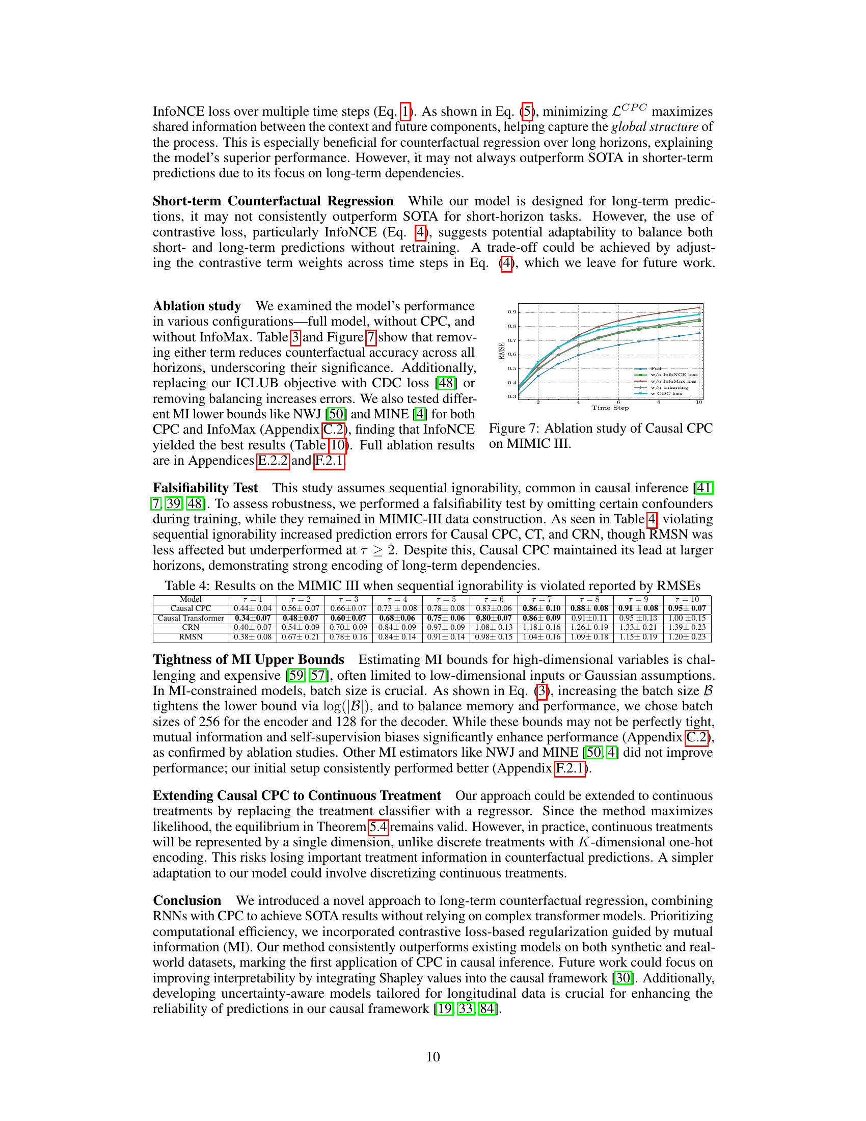
This table presents the results of experiments conducted on the MIMIC III dataset when the assumption of sequential ignorability is violated. The table shows the normalized root mean squared error (NRMSE) for different forecasting horizons (τ = 1 to τ = 10) and for four different models: Causal CPC, Causal Transformer, CRN, and RMSN. The NRMSE values demonstrate the impact of violating the sequential ignorability assumption on the accuracy of counterfactual estimation by each model over different time horizons.

This table compares Causal CPC with other state-of-the-art (SOTA) methods for counterfactual regression over time. It highlights key architectural differences, such as the model backbone (e.g., GRU, Transformer, LSTM), whether the model is explicitly designed for long-term forecasting, the use of contrastive learning, the method used to predict counterfactuals, how selection bias is handled, and whether the model ensures invertibility of the representation. This comparison helps to contextualize Causal CPC’s novel contributions and its advantages over existing approaches.
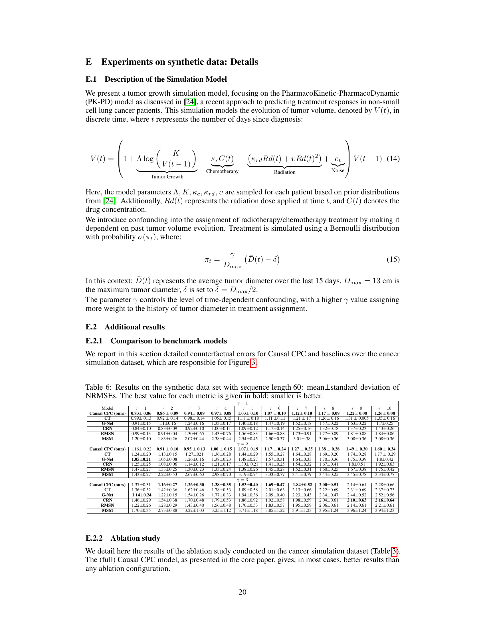
This table presents the results of the cancer simulation experiment for sequence length 60. It compares the performance of Causal CPC against other state-of-the-art models across multiple prediction horizons (τ = 1 to 10) and three different confounding levels (γ = 1, 2, 3). The performance metric is Normalized Root Mean Squared Error (NRMSE), with lower values indicating better performance. The best performing model for each scenario is highlighted in bold.

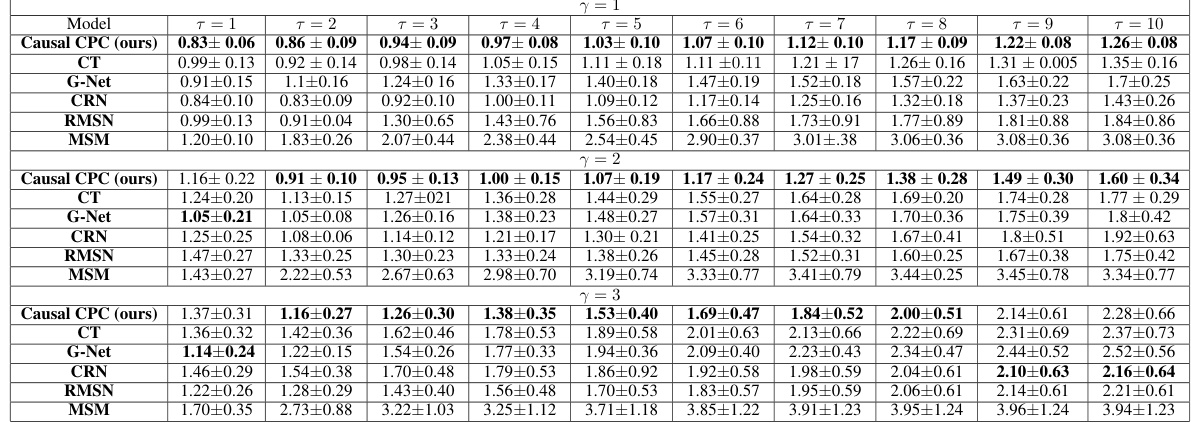
This table presents the Root Mean Squared Errors (RMSEs) for the semi-synthetic MIMIC III dataset with a sequence length of 100. It shows the RMSE values for different prediction horizons (T=1 to T=10) for the Causal CPC model and four other comparison models: CT, G-Net, CRN, and RMSN. Lower RMSE values indicate better model performance. The results are averaged across multiple runs, with standard deviations reported as well, reflecting the variability in model performance across different runs.

This table presents the results of the ablation study performed on the synthetic dataset using a sequence length of 40. The table shows the mean and standard deviation of the Normalized Root Mean Squared Errors (NRMSEs) for different horizons (τ = 1 to 10) for various model configurations: Causal CPC (full), Causal CPC without InfoNCE loss, Causal CPC without InfoMax loss, Causal CPC with CDC loss, and Causal CPC without balancing. The best NRMSE value for each horizon and each model is highlighted in bold.

This table presents the results of the semi-synthetic MIMIC III experiment, focusing on the evolution of Root Mean Squared Errors (RMSEs) across different prediction horizons (τ = 1 to 10). The experiment uses a sequence length of 100. The RMSEs are shown for Causal CPC and several other comparative models.

This table presents a comparison of the performance of the Causal CPC model using different mutual information (MI) lower bounds for contrastive predictive coding (CPC) and InfoMax. It shows the Normalized Root Mean Squared Errors (NRMSEs) for different prediction horizons (τ = 1 to 10) on the MIMIC III semi-synthetic dataset. The results demonstrate the impact of the choice of MI estimation method on model performance.

This table presents the mean and standard deviation of Root Mean Squared Errors (RMSEs) for the semi-synthetic MIMIC III dataset across different prediction horizons (τ = 1 to 10). The results are broken down by model and show the performance of Causal CPC (ours), CT, G-Net, CRN, RMSN, and MSM. A sequence length of 100 was used for this experiment. Lower RMSE values indicate better model performance.

This table compares the model complexity (in terms of trainable parameters) and the running time (in minutes) for different models, namely Causal CPC and four baselines (CT, G-Net, CRN, RMSN). The results are averaged over five runs, for a specific configuration of the tumor growth simulation (γ=1). The hardware used is a single NVIDIA Tesla M60 GPU. The table highlights that Causal CPC offers a good balance between model complexity and computational efficiency.

This table summarizes the key differences between Causal CPC and other state-of-the-art methods for counterfactual regression over time used in the paper’s experiments. It compares model backbones, ability to handle long-term forecasting, use of contrastive learning, mechanisms for handling selection bias and representation invertibility.

This table summarizes the key characteristics of the counterfactual regression models used in the paper’s experiments, including the model backbone, whether they are tailored for long-term forecasting, their handling of time-dependent confounding and selection bias, the use of contrastive learning, and whether the representation is invertible. It highlights the differences between the proposed Causal CPC model and existing state-of-the-art methods.
This table summarizes the key differences between Causal CPC and the baseline models used in the experiments. It highlights the model backbone, ability to handle long-term forecasting, use of contrastive learning, and the methods used to learn long-term dependencies, handle selection bias, and ensure the invertibility of the representation.
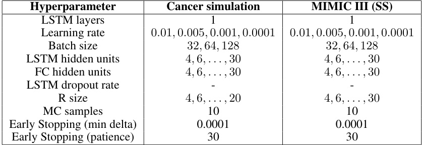
This table shows the hyperparameter search ranges used for training the Recurrent Marginal Structural Networks (RMSN) model. It details the ranges explored for various hyperparameters related to the LSTM layers (recurrent neural network layers) within the propensity and treatment networks, including the number of layers, learning rate, batch size, hidden unit count, dropout rate, and early stopping criteria. Separate ranges are provided for cancer simulation data and semi-synthetic MIMIC-III data.

This table details the hyperparameter search ranges used for training the Recurrent Marginal Structural Networks (RMSNs) model. It shows the range of values explored for various hyperparameters within the RMSN model, broken down by sub-model (Propensity Treatment Network, Propensity History Network, Encoder, Decoder) for both cancer simulation and semi-synthetic MIMIC-III datasets. The hyperparameters covered include the number of LSTM layers, learning rate, batch size, LSTM hidden units, LSTM dropout rate, maximum gradient norm, early stopping minimum delta, and early stopping patience. Each sub-model has its own set of hyperparameter ranges, demonstrating the complexity of tuning the RMSN model for optimal performance.

This table displays the hyperparameter search ranges used for the CRN model in the experiments. It breaks down the hyperparameters for the encoder and decoder sub-models separately, specifying the ranges explored for parameters like the number of LSTM layers, learning rate, batch size, LSTM hidden units, LSTM dropout rate, BR size, and early stopping criteria for both cancer simulation and MIMIC III (semi-synthetic) datasets.
This table details the hyperparameter search ranges used for training the Recurrent Marginal Structural Networks (RMSN) model. It breaks down the hyperparameters by sub-model (Propensity Treatment Network, Propensity History Network, Encoder, Decoder) and lists the range of values tested for cancer simulation and MIMIC III (SS) datasets. Each sub-model shows various tunable parameters including the number of LSTM layers, learning rate, batch size, hidden units, dropout rate, max gradient norm, and early stopping criteria (min delta and patience).
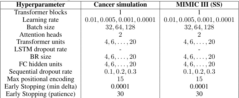
This table presents the hyperparameter search ranges used for the Causal Transformer model in the experiments. It shows the ranges explored for various parameters such as the number of transformer blocks, learning rate, batch size, number of attention heads, transformer units, LSTM dropout rate, BR size, fully connected hidden units, sequential dropout rate, maximum positional encoding, and early stopping parameters (minimum delta and patience). Separate ranges are given for the experiments conducted on the cancer simulation dataset and the semi-synthetic MIMIC III dataset.
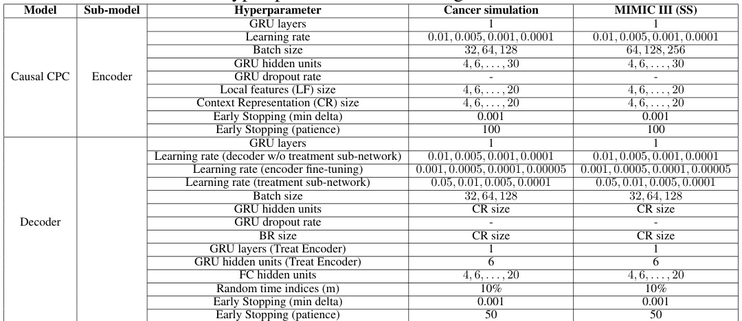
This table details the hyperparameter search ranges used for training the Recurrent Marginal Structural Networks (RMSNs) model. It covers hyperparameters for various sub-models within RMSN, including the propensity treatment network, propensity history network, encoder, and decoder. Each hyperparameter is listed along with the tested values for both the cancer simulation dataset and the semi-synthetic MIMIC-III dataset. Note that this is a search range, not all listed values were necessarily used in the final model.

This table presents the hyperparameter search ranges used for training the Recurrent Marginal Structural Networks (RMSNs) model. It includes the hyperparameters for the propensity treatment network, propensity history network, encoder, and decoder. The search ranges are provided separately for the cancer simulation and MIMIC III semi-synthetic datasets. For each hyperparameter, the table specifies the possible values explored during the hyperparameter search.
Full paper#
