↗ OpenReview ↗ NeurIPS Homepage ↗ Chat
TL;DR#
Many machine learning problems involve optimizing multiple, often conflicting objectives. Existing methods for preference-guided multi-objective learning are often limited in their flexibility or lack strong theoretical guarantees. This creates challenges in finding optimal solutions that balance different objectives according to user preferences. This paper introduces FERERO, which addresses these issues.
FERERO casts preference-guided multi-objective learning as a constrained vector optimization problem. It incorporates two types of preferences: relative preferences defined by partial ordering, and absolute preferences defined by constraints. Convergent algorithms are developed, including a novel single-loop primal algorithm, allowing for adaptive adjustment to both constraints and objective values. The effectiveness of FERERO is demonstrated through experiments on various benchmark datasets, showing its competitiveness in finding preference-guided optimal solutions.
Key Takeaways#
Why does it matter?#
This paper is important because it offers a flexible and efficient framework for preference-guided multi-objective learning. It addresses limitations of existing methods by allowing for flexible preference definitions and providing provably convergent algorithms. This opens avenues for improved solutions in various machine learning tasks involving multiple, often competing, objectives.
Visual Insights#

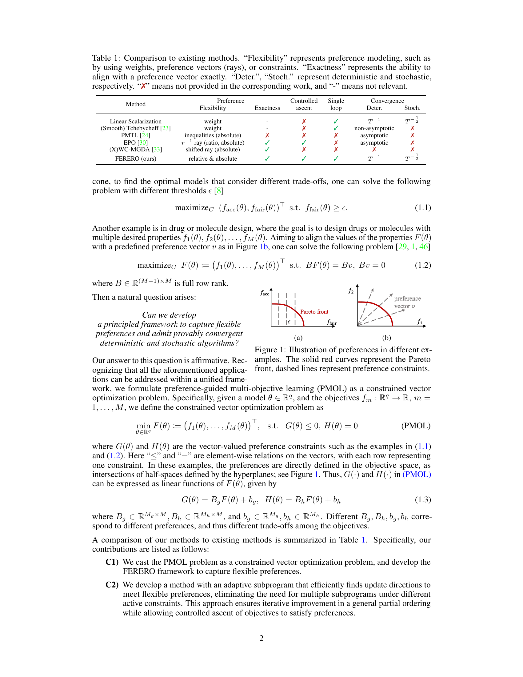
This figure illustrates two examples of how preferences are incorporated into multi-objective optimization problems. The first example (a) shows a trade-off between fairness and accuracy in machine learning. The Pareto front represents the set of optimal solutions balancing these objectives, while preference constraints (dashed lines) specify desired minimum levels of fairness (epsilon). The second example (b) illustrates drug molecule design, where a preference vector (v) guides the optimization towards solutions with specific property combinations, aligning with a particular direction in the objective space.

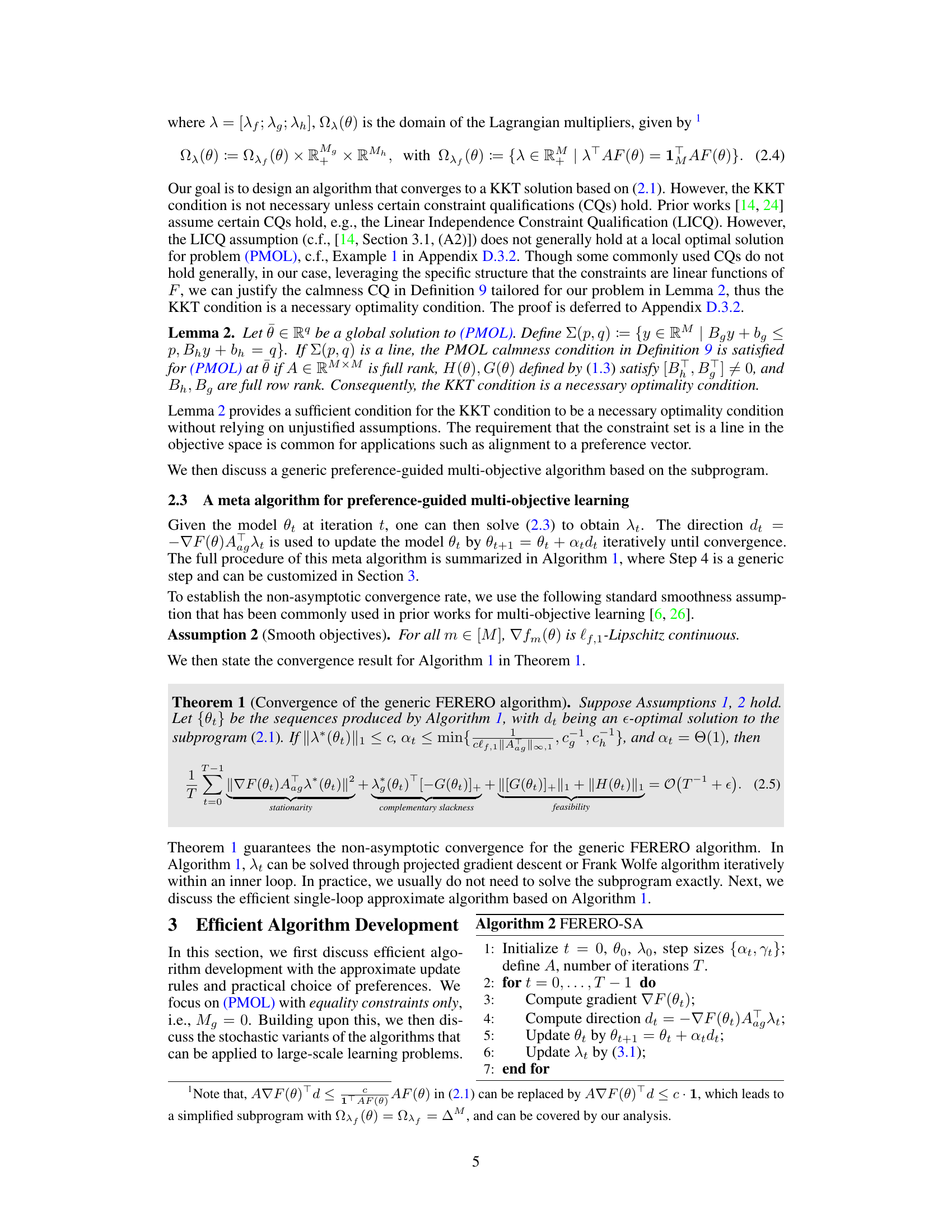
This table compares FERERO with other existing preference-guided multi-objective learning methods. It assesses the methods across several key criteria: the flexibility of their preference modeling (weights, vectors, constraints), their ability to exactly align with a specified preference, whether they use a controlled ascent strategy, if they have a single-loop algorithm, and finally, their convergence guarantees (deterministic and stochastic). The table helps to highlight the advantages and unique aspects of the FERERO framework.
In-depth insights#
Flexible PMOL#
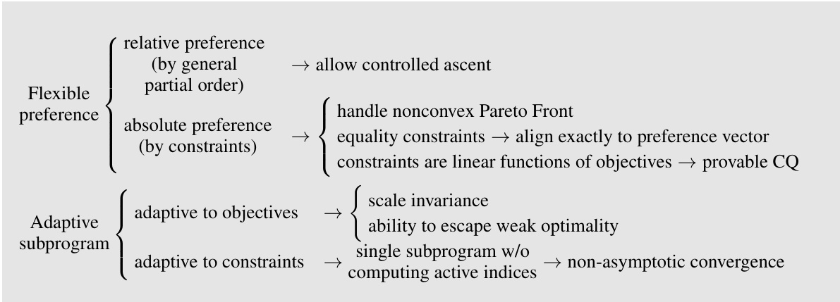
Flexible Preference-Guided Multi-Objective Learning (PMOL) represents a significant advancement in handling complex optimization problems. The flexibility lies in its capacity to incorporate diverse preference structures, moving beyond simplistic weighting schemes. This allows for a more nuanced control over the trade-offs between multiple objectives. The framework’s adaptability is further enhanced by its ability to handle both relative and absolute preferences simultaneously, offering a more comprehensive approach to guiding the optimization process towards desirable solutions. Provably convergent algorithms, both deterministic and stochastic, provide theoretical guarantees, increasing the trustworthiness and reliability of the method. The single-loop primal algorithm offers a practical advantage in computational efficiency. Overall, Flexible PMOL provides a powerful and versatile tool for tackling real-world multi-objective problems where precise control over solution characteristics is paramount.
Single-loop Alg.#
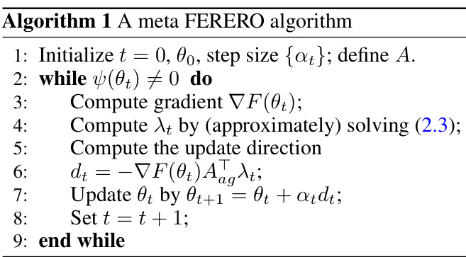
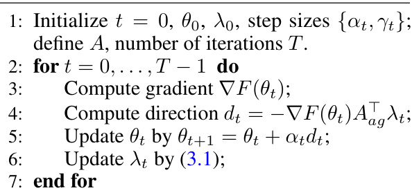
The heading ‘Single-loop Alg.’ likely refers to a novel algorithm presented in the paper for preference-guided multi-objective learning. A single-loop algorithm is computationally efficient compared to multi-loop approaches because it avoids nested optimization procedures, and thus reduces computational complexity. The authors likely demonstrate that this single-loop algorithm, despite its simplicity, achieves convergence towards optimal solutions, and possibly under specific conditions, demonstrate non-asymptotic convergence guarantees. This is a significant contribution because many existing methods in multi-objective optimization only guarantee asymptotic convergence which is not computationally feasible, especially for high-dimensional problems. The algorithm’s design likely involves adaptively adjusting to both objective and constraint values. The single-loop nature simplifies the algorithm making it more practical and easier to implement compared to nested algorithms that can be computationally expensive and complex to implement.
Adaptive PMOL#
Adaptive PMOL (Preference-guided Multi-Objective Learning) signifies a significant advancement in tackling real-world multi-objective problems. The “adaptive” nature likely refers to the algorithm’s dynamic adjustment to changing problem conditions. This could involve adaptively adjusting preferences as new information becomes available or modifying optimization strategies based on the current search progress, ensuring efficient exploration of the Pareto frontier. A key advantage would be its ability to handle diverse preference structures, moving beyond the limitations of simpler preference models. Provably convergent algorithms are crucial for such an approach, guaranteeing reliable and efficient convergence to optimal solutions. The flexibility of Adaptive PMOL makes it particularly suitable for complex applications where objective trade-offs and preferences are fluid, allowing for better alignment with specific user requirements and dynamic environmental changes.
Convergence Rates#
Analyzing convergence rates in machine learning algorithms is crucial for understanding their efficiency and reliability. Faster convergence means quicker training and potentially reduced computational costs. The theoretical analysis often provides asymptotic rates, describing the algorithm’s behavior as the number of iterations approaches infinity. However, non-asymptotic rates are more practical, offering bounds on the error after a finite number of steps, providing a measure of real-world performance. The tightness of these bounds also matters—a tighter bound offers a more precise prediction of the algorithm’s convergence speed. Furthermore, comparing different algorithms based solely on asymptotic rates can be misleading; practical performance can vary considerably due to factors such as constants and problem-specific characteristics. Therefore, a comprehensive analysis should include both asymptotic and non-asymptotic rates, acknowledging the limitations of each and considering empirical observations to gain a complete picture of the algorithm’s convergence behavior. The type of convergence—whether it’s convergence to a stationary point, a global optimum, or a KKT point—is also important when assessing the results.
Future Work#
Future research directions stemming from this paper could involve several key areas. First, extending the theoretical analysis to cover more general types of constraints beyond the linear constraints considered here is crucial. Second, developing more efficient algorithms for solving the constrained vector optimization problem, possibly through advanced optimization techniques or approximation methods, would be highly valuable. This could involve exploring alternative single-loop algorithms or adapting stochastic methods for increased scalability and efficiency. Third, a more extensive evaluation on real-world datasets with diverse characteristics is needed to further validate the proposed framework’s generalizability and robustness. Finally, it would be beneficial to explore applications in other domains. The paper’s core methodology has potential value in various fields; further investigation into specific application areas would broaden its impact and demonstrate its practical utility.
More visual insights#
More on figures
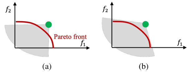
This figure illustrates the concept of CA-dominance, a generalization of Pareto dominance. In (a), the standard Pareto dominance is shown, where a point dominates another if it is better in all objectives. The gray shaded area represents the points dominated by the reference point. In (b), a more general cone (CA) is used to define dominance. This allows for more flexibility in defining preferences. The gray shaded area now encompasses a broader range of points than in (a), showing that CA-dominance can capture more diverse preference structures.

This figure compares the performance of different multi-objective optimization methods on a synthetic problem with two objectives. The goal is to find solutions that align with pre-specified preference vectors, represented by dashed arrows. The blue dots show the final solutions found by each method, while the blue lines trace their optimization trajectories. The green dots indicate the starting point of the optimization process. The figure demonstrates how different methods converge to different parts of the Pareto front, highlighting the unique capabilities of the FERERO framework.

This figure compares the performance of various multi-objective optimization methods when the initial objective values are close to the Pareto front. Each color represents a different preference, and the colored lines show the optimization trajectory of each method. The figure illustrates how each method approaches and converges to the Pareto front, highlighting differences in efficiency and ability to align with specified preferences.
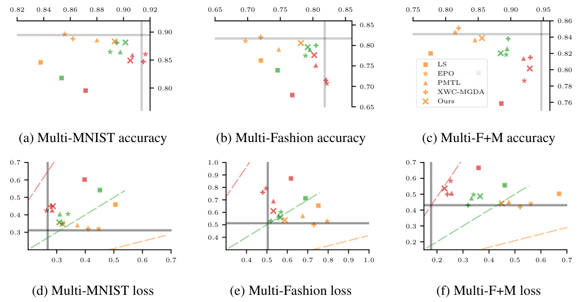
This figure shows the training losses and accuracies of different multi-objective optimization methods on three image datasets (Multi-MNIST, Multi-Fashion, and Multi-F+M). Each subplot represents a dataset, with the horizontal and vertical axes showing the results for objective 1 and objective 2, respectively. Different colored dashed arrows represent predefined preferences, and different colored markers represent the results obtained by different methods. The marker color corresponds to the preference being targeted. The results illustrate how each method performs in finding solutions that align with different preferences.

This figure shows the training losses and accuracies for three multi-objective image classification datasets (Multi-MNIST, Multi-Fashion, Multi-F+M). Each subplot represents a dataset and displays the performance of different algorithms (LS, EPO, PMTL, XWC-MGDA, and FERERO) in terms of accuracy and loss for two objectives. Different colored markers represent different algorithms, and dashed arrows show the direction of the specified preferences. The plot illustrates how well each algorithm can achieve a target preference.

This figure compares the performance of various multi-objective optimization methods on a synthetic dataset. Each method starts at the same initial point (green dot) and aims to find an optimal solution guided by a specific preference vector (dashed arrows). The blue dots represent the final solutions found by each algorithm, and the blue lines show their optimization trajectories. The plot shows how different algorithms navigate the objective space, highlighting the differences in their convergence behavior and ability to reach preference-guided solutions.

This figure demonstrates the scale invariance property of the proposed FERERO algorithm. The left subplot shows the optimization trajectory without scaling, while the right subplot shows the trajectory with scaling applied to one of the objectives. The results show that the algorithm’s convergence and preference alignment are not affected by the scaling, which demonstrates its robustness and ability to handle various scales of objective functions.
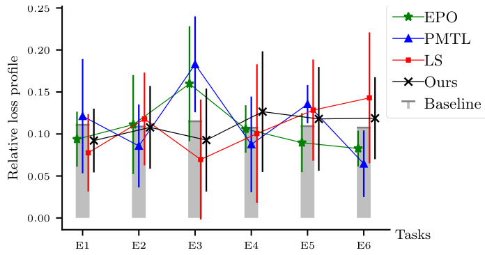
This figure compares different preference-guided multi-objective optimization methods’ performance on the Emotions and Music dataset. The x-axis represents the six different emotion categories (E1-E6). The y-axis displays the relative loss profile, which quantifies the alignment between the obtained solutions and the predefined preferences. The error bars represent the standard deviation over multiple runs. The figure allows for a visual assessment of how well each method aligns its solutions with the specified preferences for each emotion category, showing which methods better satisfy user-defined trade-offs across multiple objectives.
More on tables
This table compares FERERO with other existing preference-guided multi-objective learning methods across several key aspects. It highlights FERERO’s flexibility in modeling preferences (using weights, vectors, or constraints), its ability to achieve exact alignment with preferences, whether it uses deterministic or stochastic approaches, and whether its convergence is guaranteed. The table reveals that FERERO is unique in its combination of features, such as flexible preference modeling, single-loop algorithm and exact alignment with preferences.
This table compares FERERO to other multi-objective optimization methods, highlighting key differences in preference modeling flexibility (using weights, vectors, or constraints), ability to exactly align with preferences, algorithm type (deterministic or stochastic), and convergence properties. It helps to understand the unique features of FERERO compared to the state-of-the-art.

This table compares the proposed FERERO framework with existing multi-objective optimization methods across several key aspects. These include the flexibility of the preference modeling techniques used (weights, vectors, or constraints), the ability to precisely align with a specified preference vector, the type of algorithm (deterministic or stochastic), and the convergence properties. The table helps to highlight FERERO’s advantages in terms of flexibility and convergence guarantees.
This table compares FERERO with other existing preference-guided multi-objective learning methods. It assesses each method’s flexibility in modeling preferences (using weights, vectors, or constraints), its ability to exactly align with a preference vector, whether it uses a deterministic or stochastic algorithm, and whether it has a single-loop convergence or a multi-loop (i.e., requires different subproblems at various stages). FERERO stands out as the only method to provide both flexibility in preference modeling, exact alignment capability, and both deterministic and stochastic single-loop convergent algorithms.

This table compares FERERO with other existing preference-guided multi-objective learning methods. It highlights key differences across several dimensions, including the flexibility of preference modeling (e.g., using weights, preference vectors, or constraints), the ability to exactly align with a preference vector, whether the method is deterministic or stochastic, whether it uses a single-loop update, and its convergence guarantees. This comparison helps establish the novelty and advantages of FERERO, particularly its flexibility in handling preferences and its convergent properties.
This table compares FERERO with other existing preference-guided multi-objective learning methods across several key aspects. These include the flexibility of the preference modeling techniques used (weights, vectors, or constraints), whether the methods can exactly align with a preference vector, whether they use deterministic or stochastic algorithms, whether they involve a single-loop update mechanism, and their convergence guarantees (asymptotic or non-asymptotic).

This table compares FERERO with other existing preference-guided multi-objective learning methods, considering various aspects like preference modeling flexibility, the ability to precisely align with preferences, algorithm type (deterministic or stochastic), single-loop convergence, and convergence guarantees. It highlights FERERO’s unique capabilities and advantages.

This table compares the proposed FERERO framework with existing multi-objective optimization methods, focusing on the flexibility of preference modeling, the ability to exactly align with a preference vector, whether the method is deterministic or stochastic, and its convergence properties. It highlights FERERO’s unique capabilities in handling both relative and absolute preferences and its non-asymptotic convergence guarantees.

This table compares FERERO with other existing preference-guided multi-objective learning methods across several key aspects. These aspects include the flexibility of the preference modeling approach (weights, vectors, or constraints), the exactness of the alignment with a given preference, whether the algorithm is deterministic or stochastic, and whether single-loop convergence is achieved. The table highlights FERERO’s advantages in its ability to model flexible preferences and achieve single-loop convergence.

This table compares the proposed FERERO framework with existing preference-guided multi-objective learning methods across several key features. These features include the flexibility of the preference modeling approach (weights, vectors, or constraints), the ability to exactly align with a preference vector, the type of algorithm used (deterministic or stochastic), and whether the algorithm is a single-loop method. The table highlights FERERO’s advantages in terms of flexibility, exactness, and algorithm design.

This table compares FERERO with other existing preference-guided multi-objective learning methods across several key aspects. These include the flexibility of the preference modeling techniques used (weights, vectors, or constraints), whether methods exactly align with a preference vector, the type of algorithm used (deterministic or stochastic, single-loop or multi-loop), and finally, whether the method has asymptotic or non-asymptotic convergence guarantees.

This table compares FERERO with other existing preference-guided multi-objective learning methods. It shows the flexibility of preference modeling (using weights, vectors, or constraints), whether the methods exactly align with a preference vector, whether they use deterministic or stochastic approaches, and whether they provide single-loop ascent and convergence guarantees.

This table compares FERERO with other existing preference-guided multi-objective learning methods based on several aspects: the flexibility of the preference modeling, the exactness of aligning with preference vectors, whether the algorithm is deterministic or stochastic, and whether it uses a single-loop or multi-loop approach. It highlights FERERO’s advantages in flexibility, exactness, and single-loop convergence.
Full paper#
