↗ OpenReview ↗ NeurIPS Homepage ↗ Chat
TL;DR#
Many machine learning problems, such as image deblurring and inpainting, are formulated as Bayesian inverse problems. Recently, denoising diffusion models (DDMs) have shown promise as effective priors due to their ability to model complex data distributions. However, using DDMs as priors leads to intricate posterior distributions that are difficult to sample from, hindering their practical application. Existing methods either involve retraining model-specific components, resulting in cumbersome procedures, or introduce approximations leading to uncontrolled errors affecting the accuracy of the samples.
This paper introduces a novel framework called Divide-and-Conquer Posterior Sampling (DCPS) to address this limitation. DCPS leverages the inherent structure of DDMs to construct a sequence of simpler, intermediate posterior distributions, guiding the sampling process towards the target posterior. This approach effectively reduces approximation errors without the need for retraining. Experiments show that DCPS outperforms existing methods in various Bayesian inverse problems, demonstrating its versatility and effectiveness across tasks such as image inpainting, super-resolution, and JPEG dequantization.
Key Takeaways#
Why does it matter?#
This paper is crucial for researchers working on Bayesian inverse problems and denoising diffusion models. It offers a novel solution to a long-standing challenge: efficiently sampling from complex posterior distributions generated by DDMs. The proposed method, Divide-and-Conquer Posterior Sampling (DCPS), significantly improves upon existing techniques by reducing approximation errors without retraining, opening avenues for further research in developing efficient posterior sampling algorithms for various inverse problems. The method’s versatility and applicability across diverse tasks (including image inpainting and super-resolution) highlight its potential for broader impact within the field.
Visual Insights#

This figure shows the first two dimensions of samples generated by six different algorithms (DCPS, DDRM, DPS, IGDM, REDDIFF, MCGDIFF) for a 25-component Gaussian mixture posterior sampling problem. The red points represent samples generated by each algorithm, and the blue points represent the true posterior samples. The figure visually compares the sample distributions generated by different algorithms with the true posterior distribution to illustrate the accuracy and efficiency of each method in approximating the true posterior.

This table presents the results of an experiment comparing the performance of different algorithms on a Gaussian Mixture model. The algorithms are evaluated using the Sliced Wasserstein (SW) distance. The table shows the 95% confidence intervals for the SW distance, providing a measure of the algorithms’ accuracy in sampling from the true posterior distribution of the model. Two different dimensions are tested (dx = 10 and dx = 100). The lower the SW distance, the better the algorithm’s performance.
In-depth insights#
DCPS Framework#
The Divide-and-Conquer Posterior Sampler (DCPS) framework offers a novel approach to address the challenges of posterior sampling in Bayesian inverse problems using Denoising Diffusion Models (DDMs) as priors. The core innovation lies in its divide-and-conquer strategy, breaking down the complex posterior into a sequence of simpler, intermediate posteriors. This decomposition significantly reduces the approximation errors inherent in existing methods, avoiding the need for computationally expensive and model-specific retraining. By leveraging the inherent structure of DDMs and employing Gaussian variational inference, DCPS efficiently guides sample generation towards the target posterior. The framework’s versatility is demonstrated across a range of Bayesian inverse problems, including image inpainting, super-resolution, and JPEG dequantization, showcasing its effectiveness and robustness compared to existing approaches.
Posterior Sampling#
Posterior sampling, a crucial aspect of Bayesian inference, is explored in this paper. The core challenge lies in the intractability of posterior distributions, especially when dealing with complex priors like those from denoising diffusion models (DDMs). The authors tackle this by proposing a novel divide-and-conquer approach. This framework cleverly structures the problem by constructing a sequence of intermediate posterior distributions, guiding the sampling process towards the final target. This is a significant improvement over existing methods that often rely on computationally expensive approximations or model-specific retraining. The divide-and-conquer strategy drastically reduces approximation errors and thus improves sampling accuracy. Gaussian variational inference is employed to efficiently approximate intractable transition densities in the process. The effectiveness of this approach is demonstrated across diverse Bayesian inverse problems, showcasing its versatility and robustness.
Approximation Errors#
Approximation errors are inherent in many machine learning algorithms, especially those dealing with complex probability distributions. In the context of Bayesian inference with denoising diffusion models (DDMs), these errors arise from the intractability of the exact posterior distribution. Existing methods often rely on simplifying assumptions or approximations that introduce uncontrolled inaccuracies. This can lead to suboptimal results or even failure to recover the underlying signal. The paper’s focus on divide-and-conquer strategies aims to mitigate these errors by breaking the problem into smaller, more manageable subproblems. By strategically managing the complexity of intermediate posterior approximations, the approach minimizes the accumulation of error across these steps. This technique contrasts with single-pass methods where errors propagate cumulatively. The effectiveness of this approach hinges on the quality of approximations in each subproblem and careful selection of intermediate distributions. The analysis of approximation errors, therefore, is crucial for evaluating the algorithm’s performance and understanding its limitations. This analysis provides theoretical guarantees and empirically supports the claim that the divide-and-conquer strategy effectively reduces approximation errors compared to existing techniques.
Experimental Results#
A thorough analysis of the ‘Experimental Results’ section requires examining the types of experiments conducted, the metrics used for evaluation, and the presentation of the results. The clarity and organization are crucial, ensuring that the results are easily understandable and support the paper’s claims. Statistical significance should be clearly demonstrated through error bars, confidence intervals, or appropriate statistical tests, which must be clearly defined. A strong results section will also include analysis, not just raw data, providing interpretations and drawing meaningful conclusions. It should compare the presented method against relevant baselines. Reproducibility is key: sufficient details on experimental setup, including data preprocessing, hyperparameters, and computational resources, must be provided to enable others to replicate the results. Finally, limitations of the experimental setup should be acknowledged, ensuring a balanced and comprehensive assessment.
Future Directions#
The ‘Future Directions’ section of this research paper would ideally delve into several crucial areas. First, it should address the limitations of the current divide-and-conquer posterior sampling (DCPS) approach, specifically its reliance on user-defined potentials. Developing a method for automatically learning or optimizing these potentials would significantly broaden the applicability and improve the generalizability of the algorithm. Second, the paper could explore extensions to more complex Bayesian inverse problems, going beyond the linear models considered and potentially examining non-linear or high-dimensional scenarios. Investigating theoretical guarantees and convergence rates for the DCPS algorithm in such settings would be particularly valuable. Third, addressing the computational cost of the algorithm warrants discussion, possibly focusing on techniques to reduce runtime and memory requirements for large-scale datasets. Lastly, exploring different types of inverse problems and demonstrating the algorithm’s effectiveness across various applications would strengthen the work and highlight its real-world potential.
More visual insights#
More on figures

This figure compares different posterior sampling algorithms on a 25-component Gaussian mixture model. The first two dimensions of the samples generated by each algorithm (DCPS, DDRM, DPS, IGDM, REDDIFF, MCGDIFF) are plotted in red, while the true samples from the posterior distribution are shown in blue. This visualization helps assess the accuracy of each algorithm by visually comparing how well their samples approximate the true posterior.

This figure shows the performance of different posterior sampling algorithms on a 25-component Gaussian mixture model. The algorithms are compared by plotting the first two dimensions of the samples generated by each method. The red dots represent samples from each algorithm (DCPS, DDRM, DPS, IGDM, REDDIFF, MCGDIFF), while the blue dots represent samples from the true posterior distribution. This visualization helps to assess the accuracy of each algorithm in approximating the true posterior distribution.

This figure compares the performance of different posterior sampling algorithms on a simple 25-component Gaussian mixture model. The algorithms are DCPS, DDRM, DPS, IGDM, REDDIFF, and MCGDIFF. The figure shows the first two dimensions of samples generated by each algorithm (in red) against the true samples (in blue). The comparison is based on a posterior sampling problem where the dimension of the signal is 100 and the dimension of the observation is 1.

This figure compares several algorithms for trajectory completion, showing their predictions for the missing part of a trajectory (the middle section). The top row shows example reconstructions of the trajectory by each algorithm, while the middle and bottom rows visualize the confidence intervals for the x and y coordinates of the predictions, respectively. The ground truth trajectory is also displayed for comparison. The dataset used is UCY, a dataset containing pedestrian trajectories.

This figure shows a comparison of different algorithms for posterior sampling on a 25-component Gaussian mixture. The algorithms include DCPS (Divide-and-Conquer Posterior Sampling), DDRM (Denoising Diffusion Restoration Models), DPS (Diffusion Posterior Sampling), IGDM (Inverse Guided Diffusion Models), REDDIFF, and MCGDIFF. The plot displays the first two dimensions of samples generated by each algorithm (in red), overlaid on the true posterior samples (in blue). This visualization allows for a qualitative assessment of each method’s accuracy in approximating the true posterior distribution.
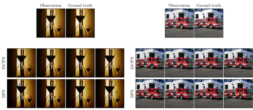
This figure shows the results of trajectory prediction using different algorithms. The top row shows the observed trajectory (incomplete) and ground truth. Subsequent rows illustrate the predictions made by two different algorithms (DCPS and DPS) at three different quantile levels (50th, 25th, and 75th). The goal is to predict the missing parts of the trajectory based on observed data.

This figure shows sample images generated by different algorithms (DCPS, DDRM, DPS, IGDM, REDDIFF, MCGDIFF) for various image restoration tasks. The tasks include inpainting with different mask types (center, half, expand) and super-resolution with upscaling factors of 4x and 16x. The results are shown for two datasets: FFHQ (left) and ImageNet (right). The purpose is to visually compare the quality of image generation across different methods.
This figure shows the result of applying different algorithms to sample from a 25-component Gaussian mixture posterior distribution in a low-dimensional space (first two dimensions are shown). The red dots represent samples generated by each algorithm (DCPS, DDRM, DPS, IGDM, REDDIFF, MCGDIFF), while blue dots represent the ground truth samples from the true posterior distribution. This visualization allows for a qualitative comparison of the algorithms’ ability to accurately capture the true posterior distribution.

This figure displays sample images generated by different algorithms (DCPS, DDRM, DPS, IGDM, REDDIFF, and MCGDIFF) for various image restoration tasks. The tasks include inpainting (with center, half, and expand masks) and super-resolution (with upscaling factors of 4x and 16x). The results are shown for two datasets: FFHQ (left) and ImageNet (right). The figure showcases the visual quality of the image reconstructions produced by each algorithm.
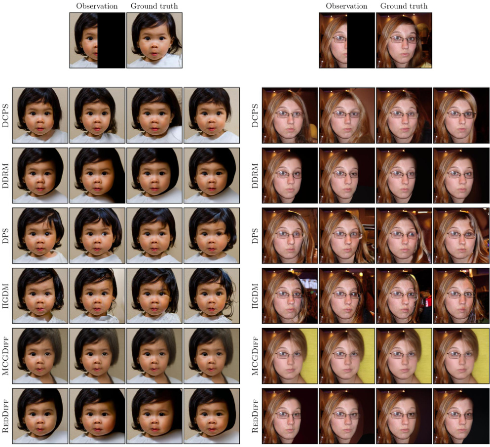
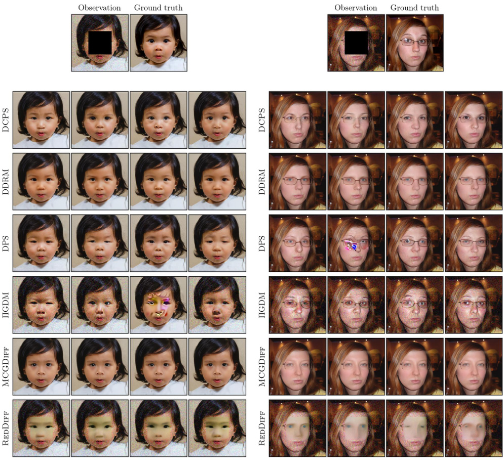
This figure shows the results of different algorithms on an inpainting task with a box mask on the FFHQ dataset. The algorithms compared are DCPS, DDRM, DPS, IGDM, MCGDIFF, and REDDIFF. Each row represents the results of one method, with four images showing different inpainting results using the same mask and seed. The first column shows the original image, with the masked region. The remaining columns show the inpainting output from the different algorithms. This allows a visual comparison of the inpainting quality and how each algorithm handles the task.
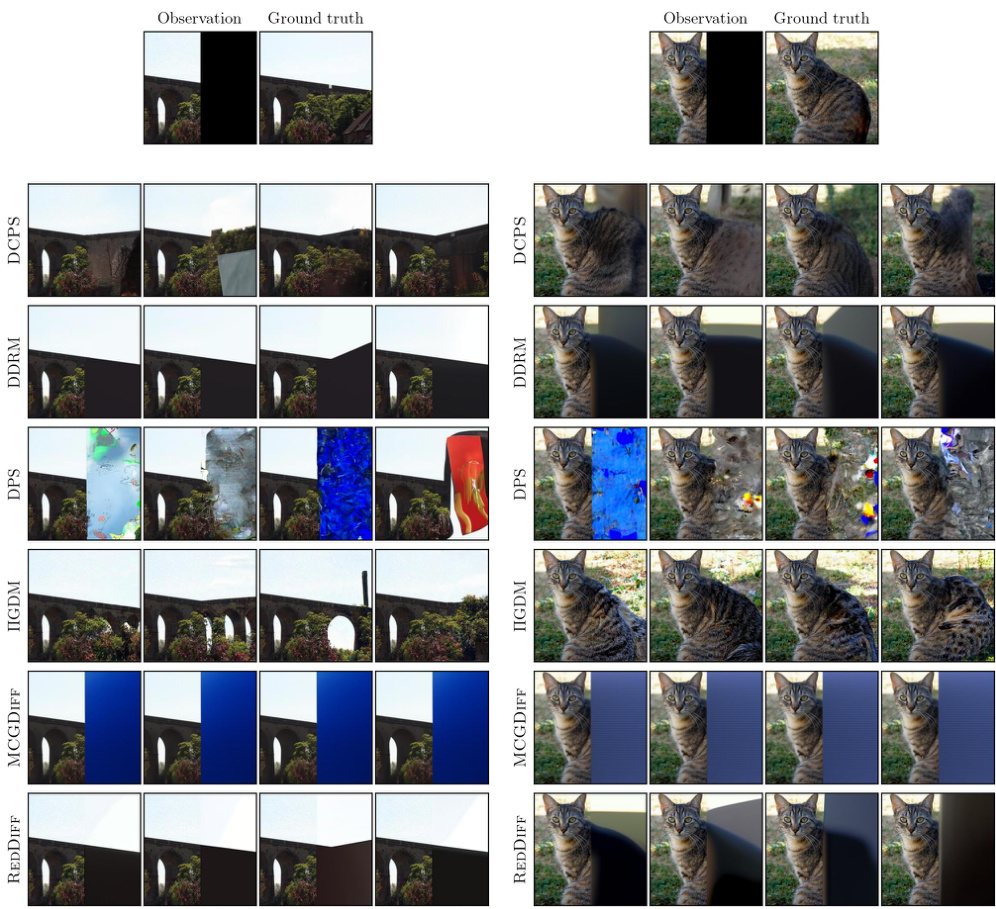
This figure shows the results of different algorithms for inpainting and super-resolution tasks using two datasets: FFHQ and ImageNet. For each task (inpainting with different mask types and 4x/16x super-resolution), sample images generated by DCPS, DDRM, DPS, IGDM, REDDIFF, and MCGDIFF are displayed side-by-side, allowing a visual comparison of their performance. The left column showcases results from the FFHQ dataset, while the right column presents results from the ImageNet dataset.

This figure compares the performance of several algorithms (DCPS, DDRM, DPS, IGDM, REDDIFF, MCGDIFF) for sampling from a 25-component Gaussian mixture posterior distribution in a 100-dimensional space. The algorithms’ samples are displayed in red, and the true posterior samples are shown in blue for comparison. It illustrates the ability of each algorithm to accurately capture the underlying distribution.
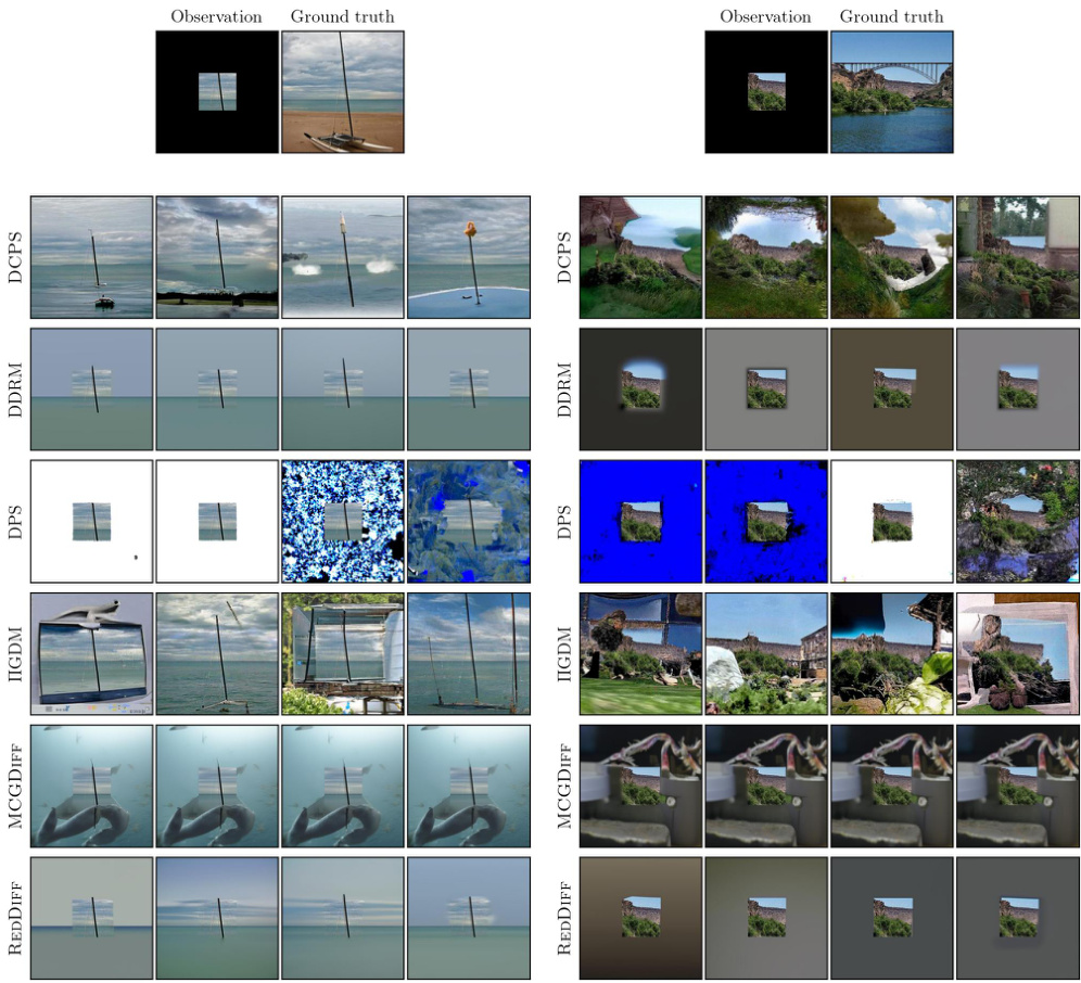
This figure shows the results of several image inpainting and super-resolution methods on two datasets (FFHQ and ImageNet). Different types of masks (center, half, expand) were used for the inpainting task, and 4x and 16x scaling factors were used for super-resolution. The results are visually compared across various algorithms: DCPS, DDRM, DPS, IGDM, REDDIFF, and MCGDIFF.

This figure visualizes the results of trajectory completion task on the UCY dataset. The top row shows the observation (incomplete trajectory) and the ground truth. The next two rows present the trajectory reconstructions generated by DCPS and MCGDIFF respectively, along with their corresponding confidence intervals. The results illustrate the performance of both algorithms in filling in missing sections of the trajectories.

This figure shows sample images generated by different algorithms for various image restoration tasks. The tasks include inpainting (with different mask types: center, half, expand) and super-resolution (upscaling by factors of 4x and 16x). The left column showcases results using the FFHQ dataset, while the right column demonstrates results from the ImageNet dataset. This visualization allows for a direct comparison of the image quality and detail produced by each method.
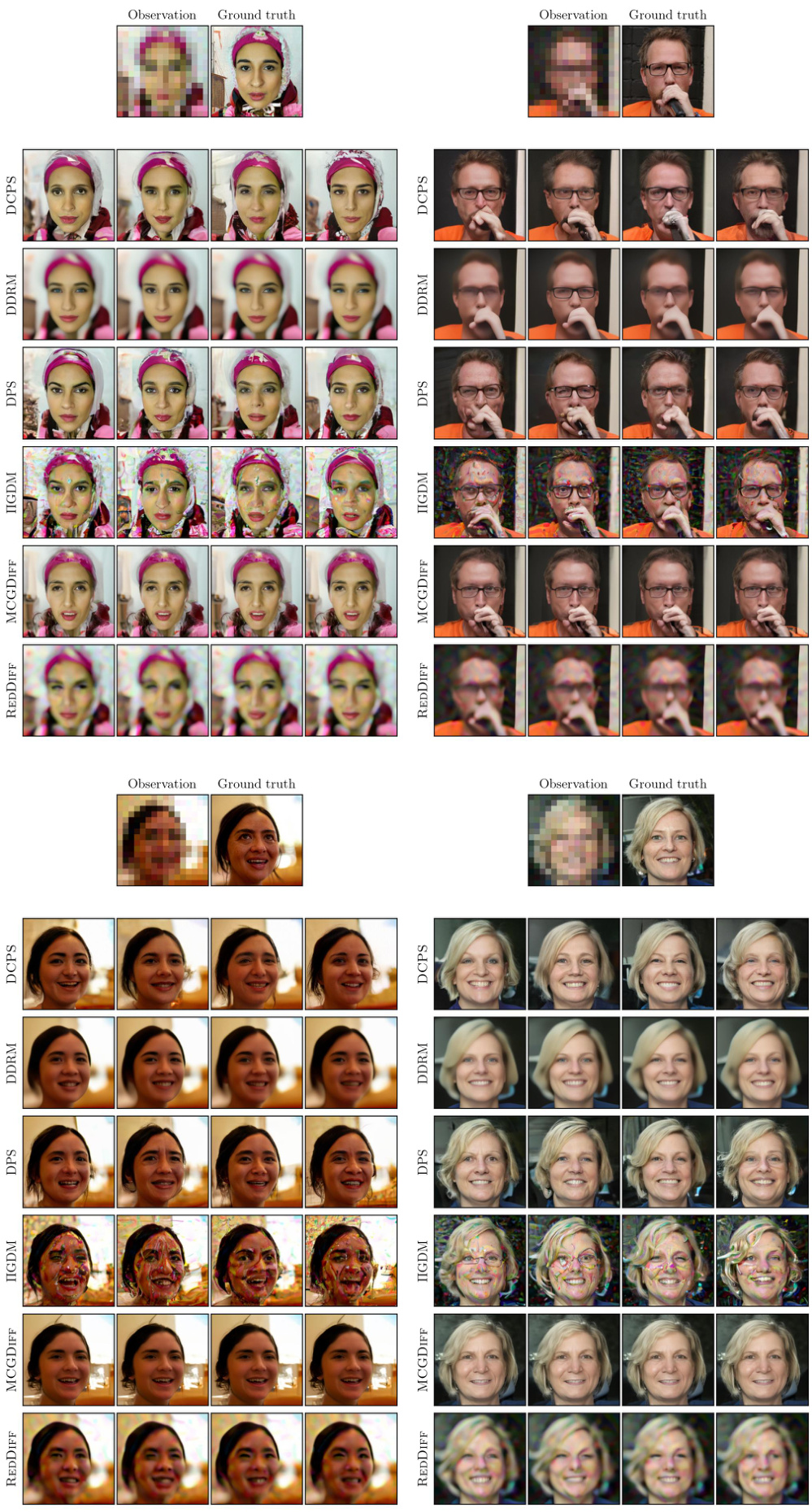
This figure shows sample images generated by different algorithms for image inpainting and super-resolution tasks. Two datasets are used: FFHQ (high-quality images of faces) and ImageNet (a large dataset of diverse images). Three different masks are used for the inpainting experiments. The algorithms are compared based on the visual quality of their generated images. This provides a visual comparison of the results of several posterior sampling algorithms on image restoration tasks.

This figure shows sample images generated by different algorithms for various image restoration tasks, including inpainting (with center, half, and expand masks) and super-resolution (4x and 16x upscaling). The results are shown for two different datasets: FFHQ (left) and ImageNet (right). The images illustrate the visual quality of the reconstructions generated by each method.
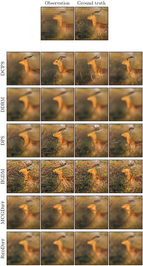
This figure shows the results of different algorithms on image inpainting and super-resolution tasks, using two datasets: FFHQ and ImageNet. For each task and dataset, sample images are displayed, illustrating the performance of each method. The figure highlights the visual differences in the quality of reconstruction between the different algorithms.

This figure shows the result of different posterior sampling algorithms on a 25-component Gaussian mixture. The x and y axes represent the first two dimensions of the samples. Red dots represent samples generated by each algorithm (DCPS, DDRM, DPS, IGDM, REDDIFF, MCGDIFF), while blue dots represent the ground truth samples from the true posterior distribution. The figure visually compares the accuracy of the different sampling algorithms by showing how close their generated samples are to the true posterior distribution.

This figure visualizes the performance of different posterior sampling algorithms on a 25-component Gaussian mixture model. The algorithms are DCPS, DDRM, DPS, IGDM, REDDIFF, and MCGDIFF. The plot shows the first two dimensions of the samples generated by each algorithm (in red) against the true posterior samples (in blue). The goal is to visually assess how well each algorithm approximates the true posterior distribution.

This figure displays sample images generated by different algorithms (DCPS, DDRM, DPS, IGDM, REDDIFF, MCGDIFF) for image inpainting and super-resolution tasks. The input images are from the FFHQ dataset (left) and the ImageNet dataset (right). Each column shows results for a different task: inpainting with center mask, inpainting with half mask, inpainting with expand mask, super-resolution 4x, and super-resolution 16x. The figure provides a visual comparison of the performance of different algorithms in handling these inverse problems.

This figure shows sample images generated by different algorithms for image inpainting and super-resolution tasks using two different datasets (FFHQ and ImageNet). Each task has different mask types or upscaling factors for super-resolution. The figure visually compares the results from several models, allowing for a qualitative assessment of their performance.
More on tables
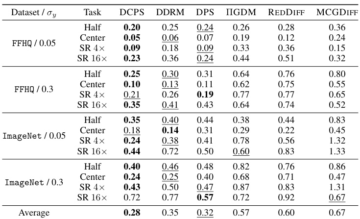
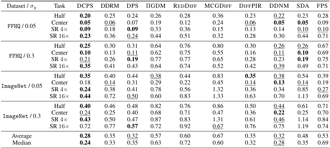
This table presents the mean Linearly Invariant Perceptual Image Patch Similarity (LPIPS) scores for different image restoration tasks (inpainting with center, half, and expand masks; super-resolution with 4x and 16x factors) and datasets (FFHQ and ImageNet). Lower LPIPS scores indicate better performance. The table compares the results of DCPS against DDRM, DPS, IGDM, REDDIFF, and MCGDIFF, showing the performance of each algorithm on various tasks and levels of noise.

This table presents the mean LPIPS (Learned Perceptual Image Patch Similarity) values achieved by different algorithms on the JPEG dequantization task. LPIPS is a perceptual metric for evaluating the quality of images, with lower values indicating better image quality. The results are shown for two datasets (FFHQ and ImageNet) and two quality factors (QF = 2 and QF = 8), representing high and low compression levels, respectively. The algorithms being compared are DCPS, IGDM, and REDDIFF.
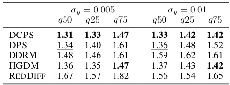
This table presents the l2 distance quantiles for trajectory prediction experiments, comparing different algorithms against MCGDIFF. The results are categorized by noise level (σy = 0.005 and σy = 0.01) and show the median (q50), 25th percentile (q25), and 75th percentile (q75) of the l2 distances. Lower values indicate better performance relative to the MCGDIFF benchmark.
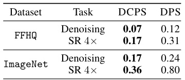
This table presents the mean LPIPS (Learned Perceptual Image Patch Similarity) values for denoising and super-resolution (SR 4x) tasks using two datasets: FFHQ and ImageNet. The LPIPS metric is used to assess the perceptual quality of image reconstruction. Lower LPIPS values indicate better reconstruction quality. The table compares the performance of the proposed DCPS algorithm with the existing DPS algorithm.
This table presents the results of an experiment comparing the performance of different posterior sampling algorithms on a Gaussian Mixture model. The algorithms are evaluated using the Sliced Wasserstein (SW) distance, a metric that measures the distance between probability distributions. The table shows the 95% confidence intervals for the SW distance for two different problem dimensions (dx = 10 and dx = 100) and includes results for DCPS (with 50 and 500 Langevin steps), DPS, DDRM, IGDM, REDDIFF, and MCGDIFF. Lower SW distance values indicate better performance.

This table presents the results of trajectory prediction experiments. It compares the performance of DCPS against other algorithms using the l2 distance. The l2 distance quantiles (q50, q25, q75) are reported for two different noise levels (σy = 0.005 and σy = 0.01). MCGDIFF serves as a reference since it asymptotically provides accurate approximations of the posterior in the trajectory prediction scenario.
Full paper#
