TL;DR#
Many combinatorial problems, such as Job Shop Scheduling (JSP), lack sufficient labeled data for supervised machine learning. Existing methods like reinforcement learning are complex and require extensive tuning. This paper introduces Self-Labeling Improvement Method (SLIM), a self-supervised approach that leverages the ability of generative models to produce multiple solutions. Instead of relying on expensive exact solutions, SLIM uses the best solution among multiple sampled ones as a pseudo-label, iteratively improving the model’s generation capability. This eliminates the need for optimal solutions and simplifies the training process.
The core contribution is the SLIM algorithm which, when used with a pointer network-based generative model, outperforms many existing heuristics and recent learning-based approaches for JSP on benchmark datasets. The method’s robustness and generality are confirmed through experiments on various instance sizes and on the Traveling Salesman Problem. This suggests SLIM is a promising general method for tackling similar combinatorial problems where labeled data is scarce.
Key Takeaways#
Why does it matter?#
This paper is important because it introduces a novel self-supervised learning method, SLIM, for training generative models to solve combinatorial optimization problems. This addresses the significant challenge of obtaining labeled data for such problems, opening new avenues for applying machine learning techniques to complex scheduling and optimization tasks. The paper’s success in solving Job Shop Scheduling problems and its adaptability to other problems like the Traveling Salesman Problem demonstrates its broad potential impact. This research is highly relevant to current trends in self-supervised learning and neural combinatorial optimization, and it offers valuable insights for researchers looking to improve the efficiency and effectiveness of these techniques.
Visual Insights#

🔼 This figure illustrates how feasible solutions for the Job Shop Problem (JSP) can be constructed step-by-step. A JSP instance is represented by a disjunctive graph (left side), showing jobs and their operations on machines. The construction process is visualized as a decision tree, where each path from the root to a leaf represents a complete solution. Each node in the tree represents a decision point, choosing which job operation to schedule next, subject to precedence constraints and machine availability (the cross symbol indicates a completed job). The colored nodes show which machine is being assigned to a job, and several feasible solutions are depicted at the bottom.
read the caption
Figure 1: The sequences of decisions for constructing solutions in a JSP instance with two jobs (J₁ and J2) and two machines (identified in green and red). Best viewed in colors.

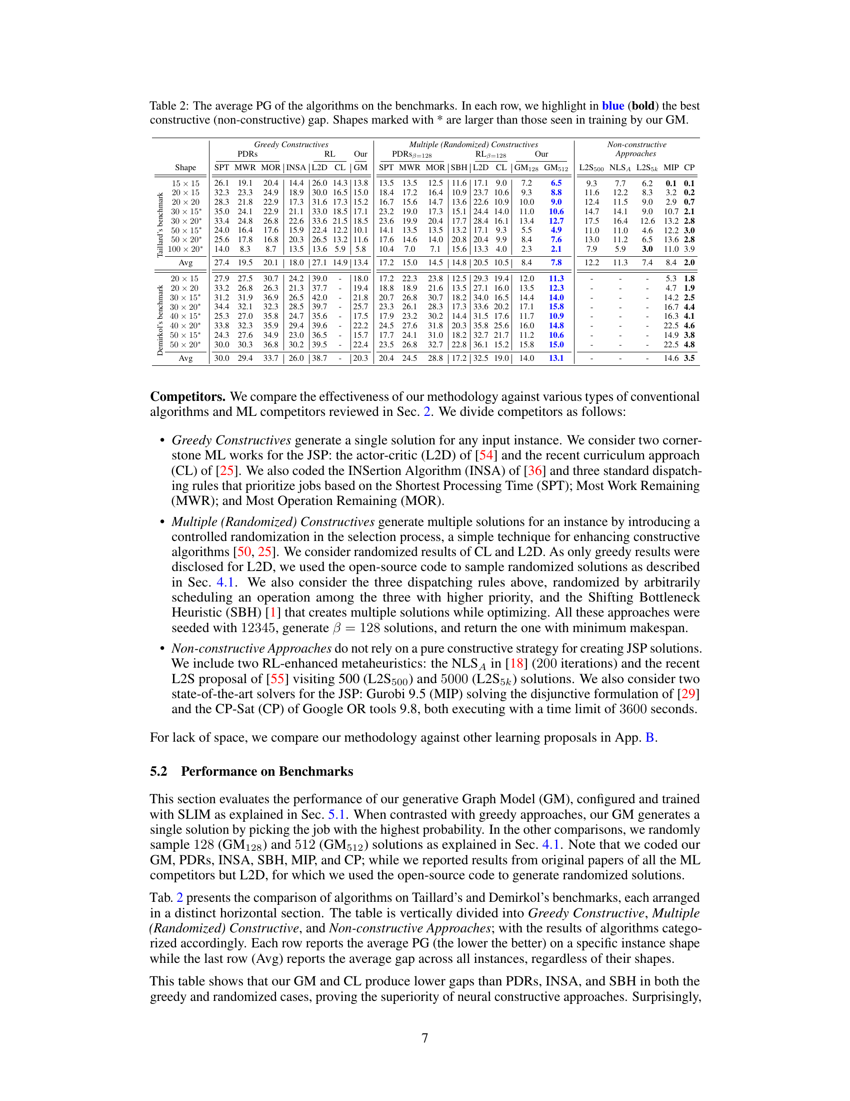
🔼 This table compares the performance of various algorithms on two benchmark datasets for the Job Shop Problem (JSP). It shows the average percentage gap (PG) for each algorithm on different problem sizes (shapes). The best constructive and non-constructive algorithms are highlighted for each shape, and shapes marked with an asterisk (*) indicate problem sizes larger than those used during the training of the generative model. The table helps illustrate the relative effectiveness of different approaches, including greedy constructive methods, multiple constructive methods, priority dispatching rules (PDRs), reinforcement learning (RL) approaches, and the proposed generative model.
read the caption
Table 2: The average PG of the algorithms on the benchmarks. In each row, we highlight in blue (bold) the best constructive (non-constructive) gap. Shapes marked with * are larger than those seen in training by our GM.
In-depth insights#
Self-Supervised JSP#
A self-supervised approach to the Job Shop Problem (JSP) offers a compelling alternative to traditional supervised methods, which often rely on expensive, optimally-solved datasets. The core idea is to leverage a generative model to produce multiple solutions for a given JSP instance and then use the best solution (according to the makespan objective) as a pseudo-label. This approach eliminates the need for external labels, thereby reducing data annotation costs and potentially improving generalization. The effectiveness hinges on the ability of the generative model to learn a meaningful representation of the JSP, enabling it to generate diverse and high-quality solutions. Furthermore, this self-supervised framework allows for iterative improvement of the model’s performance, allowing the algorithm to learn from its mistakes and progressively refine its solution-generating capability. The approach shows promise as it can potentially bypass the computational constraints associated with traditional methods, making it suitable for larger and more complex JSP instances. However, it is important to consider the limitations inherent in relying solely on self-supervision, including the potential for the model to get stuck in local optima and the need for careful parameter tuning to achieve optimal performance. Future work could explore strategies for enhancing exploration-exploitation balance in the generative model and rigorously comparing its performance against other self-supervised and reinforcement learning techniques.
SLIM’s Robustness#
The robustness of the Self-Labeling Improvement Method (SLIM) is a crucial aspect to evaluate. Its effectiveness hinges on the balance between exploration and exploitation during solution generation. SLIM’s reliance on pseudo-labels derived from the best sampled solution introduces a potential bias, impacting generalization. Experiments should rigorously explore the sensitivity of performance to variations in the number of sampled solutions. A sensitivity analysis on hyperparameters such as the sampling strategy and network architecture is also necessary to understand SLIM’s limitations and ensure reliable performance across different problem instances. Further investigations into the effect of instance characteristics on SLIM’s performance could reveal its true robustness and adaptability to various problem domains. The impact of the initial model configuration also requires further attention, as the effectiveness of SLIM may depend on a carefully selected initial model. Overall, a comprehensive assessment of SLIM’s robustness should systematically assess these factors to provide a complete picture of its reliability and generalizability.
Generative Model#
A generative model, in the context of a research paper on combinatorial optimization problems, is a crucial component for efficiently exploring the solution space. It learns the underlying structure of the problem to generate multiple potential solutions. This contrasts with traditional methods which might focus on a single solution path. The model’s effectiveness hinges on its ability to sample solutions of varying quality, enabling the selection of high-quality solutions via a self-supervised approach. Key to the success of a generative model is its architecture, typically involving an encoder to process problem-specific data and a decoder to generate solutions sequentially. The training strategy employed is also crucial, leveraging techniques like self-labeling to improve the model’s ability to create good solutions without the need for expensive human labeling. Ultimately, a well-designed generative model offers a powerful and scalable tool for tackling complex combinatorial problems, surpassing traditional heuristics in speed and/or solution quality.
TSP Application#
A hypothetical ‘TSP Application’ section in a research paper could explore using Traveling Salesperson Problem (TSP) algorithms to solve real-world optimization challenges. It might delve into specific applications like route optimization for delivery services, network design in telecommunications, or robotic path planning. The discussion would likely focus on adapting standard TSP algorithms (e.g., heuristics, approximation algorithms) or exploring novel approaches tailored to the specific constraints and characteristics of the application domain. Benchmarking results against existing solutions would demonstrate the effectiveness and scalability of the proposed method. A key aspect would be analyzing how the complexity and problem size of the real-world application translate into computational demands and performance trade-offs. The section might also highlight the limitations of using a TSP framework to model the application, such as ignoring real-world factors like traffic congestion or time windows.
Future of SLIM#
The future of SLIM (Self-Labeling Improvement Method) looks promising due to its minimal assumptions and ease of implementation. Its self-supervised nature reduces reliance on costly labeled data, a significant advantage for combinatorial optimization. Future research could explore hybrid approaches, combining SLIM with reinforcement learning or other methods to improve efficiency and potentially address limitations such as the reliance on selecting only the single best solution during training. Investigating different sampling strategies, beyond simple random sampling, to enhance performance is another promising avenue. Furthermore, the generality of SLIM could be tested on a broader range of combinatorial problems, exploring its effectiveness in areas like graph optimization and resource allocation. Addressing the memory constraints associated with parallel solution generation is crucial for scalability. Developing techniques to efficiently generate higher-quality solutions with reduced memory footprint will be key to deploying SLIM on larger, more complex problems. Finally, understanding SLIM’s theoretical guarantees and its connection to existing optimization methods would offer deeper insights and potentially lead to further improvements.
More visual insights#
More on figures

🔼 This figure shows the validation curves of a generative model (GM) for the Job Shop Scheduling Problem (JSP) when trained using two different methods: Proximal Policy Optimization (PPO) and the proposed Self-Labeling Improvement Method (SLIM). The y-axis represents the average percentage gap (PG) on the Taillard benchmark dataset, which measures the difference between the obtained makespan and the optimal makespan. The x-axis shows the training step. The figure demonstrates that SLIM achieves faster convergence and better performance compared to PPO, as indicated by lower PG values and a steeper descent of the curve. The results highlight the effectiveness of SLIM in training generative models for combinatorial optimization problems.
read the caption
Figure 2: GM validation curves when trained with PPO and our SLIM in the same training setting of [54].

🔼 The figure shows the validation curves of a generative model (GM) trained with Proximal Policy Optimization (PPO) and Self-Labeling Improvement Method (SLIM) on the Taillard benchmark. The x-axis represents training steps, and the y-axis represents the average Percentage Gap (PG). The graph compares the performance of the GM trained with PPO and SLIM, demonstrating that SLIM leads to faster convergence and better final model performance.
read the caption
Figure 2: GM validation curves when trained with PPO and our SLIM in the same training setting of [54].

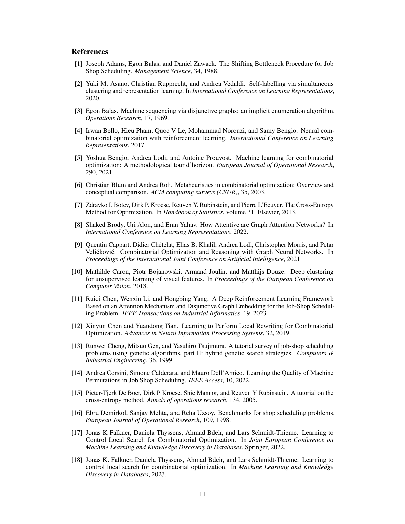
🔼 The figure shows the validation curves for training a neural network model for the Traveling Salesman Problem (TSP) using two different training methods: SLIM (Self-Labeling Improvement Method) and POMO (Policy Optimization with Multiple Optima). The y-axis represents the average optimality gap on the TSPLIB benchmark, while the x-axis represents the training step. The curves show that SLIM achieves faster convergence than POMO and reaches a similar level of performance as the best POMO model (POMO20) from a previous study. This demonstrates that SLIM is an effective training strategy for TSP, a challenging combinatorial optimization problem.
read the caption
Figure 5: Validation curves obtained by training with SLIM and POMO on random TSP instances with 20 nodes. POMO20 is the best model produced in [30], trained on instances with 20 nodes.

🔼 This figure shows the validation curves of a generative model (GM) trained using two different methods: Proximal Policy Optimization (PPO) and the proposed Self-Labeling Improvement Method (SLIM). The x-axis represents the training step, and the y-axis represents the average percentage gap (PG) on the Taillard benchmark. The graph compares the performance of GM trained with PPO and SLIM with different numbers of sampled solutions (β). The results demonstrate that SLIM leads to faster convergence and produces better final models compared to PPO.
read the caption
Figure 2: GM validation curves when trained with PPO and our SLIM in the same training setting of [54].
More on tables
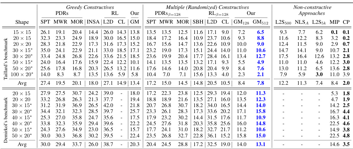
🔼 This table presents the average percentage gap (PG) of different algorithms on two benchmark datasets (Taillard’s and Demirkol’s) for job shop scheduling. It compares several approaches: greedy constructive heuristics (simple methods for generating solutions), multiple randomized constructive heuristics (improving solutions by adding randomness), and non-constructive methods (more complex, non-heuristic methods). The table is organized by shape (size of the problem) and highlights the best-performing algorithm for each shape, categorized as either constructive (building a solution step-by-step) or non-constructive. Shapes marked with an asterisk (*) indicate problem sizes larger than those seen during the training of the generative model (GM). The table allows comparison of different solution generation strategies.
read the caption
Table 2: The average PG of the algorithms on the benchmarks. In each row, we highlight in blue (bold) the best constructive (non-constructive) gap. Shapes marked with * are larger than those seen in training by our GM.
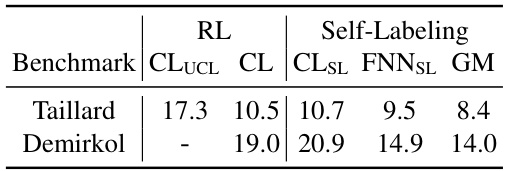
🔼 This table compares the average performance gaps of different models on Taillard and Demirkol benchmarks. The models are trained using different methods: reinforcement learning (RL) with and without curriculum learning, and self-labeling. The results show that the self-labeling approach leads to lower gaps (better performance).
read the caption
Table 3: The average gaps when sampling 128 solutions from architectures trained without and with self-labeling. CLUCL is the model obtained in [25] by training with reward-to-go on random instance shapes (no curriculum learning) and CL is similarly obtained by applying curriculum learning.

🔼 This table lists 11 features used to create a context vector for each job within a partial solution during the construction of a solution for the Job Shop Problem (JSP). Each feature provides information about the job’s status relative to the current partial solution and its remaining operations, including completion times and comparisons to averages and quartiles.
read the caption
Table 1: The features of a context vector cj ∈ R11 that describes the status of a job j within a partial solution π

🔼 This table compares the performance of various algorithms on two benchmark datasets (Taillard’s and Demirkol’s) for the Job Shop Problem (JSP). It shows the average percentage gap (PG) for each algorithm on different problem instance sizes (shapes). The best-performing constructive (single-solution) and non-constructive (multiple-solution) algorithms are highlighted for each shape. The asterisk (*) indicates problem shapes larger than those used for training the generative model (GM). This allows assessment of the GM’s generalization capabilities.
read the caption
Table 2: The average PG of the algorithms on the benchmarks. In each row, we highlight in blue (bold) the best constructive (non-constructive) gap. Shapes marked with * are larger than those seen in training by our GM.

🔼 This table presents the average percentage gap (PG) achieved by various algorithms on two benchmark datasets: Taillard’s and Demirkol’s. The algorithms are categorized into greedy constructive, multiple (randomized) constructive, and non-constructive approaches. The table highlights the best-performing constructive and non-constructive algorithms for each instance shape, offering a comparative analysis of different algorithmic approaches on the JSP problem.
read the caption
Table 2: The average PG of the algorithms on the benchmarks. In each row, we highlight in blue (bold) the best constructive (non-constructive) gap. Shapes marked with * are larger than those seen in training by our GM.

🔼 This table presents the average percentage gap (PG) for various algorithms on two benchmark datasets (Taillard and Demirkol). It compares the performance of several constructive heuristics (greedy and randomized), priority dispatching rules (PDRs), reinforcement learning (RL) approaches, and the proposed generative model (GM). The table is organized to show separate results for constructive methods and non-constructive methods, highlighting the best performing algorithm for each instance shape in both categories. The asterisk (*) indicates that some instance shapes are larger than those used in training the generative model.
read the caption
Table 2: The average PG of the algorithms on the benchmarks. In each row, we highlight in blue (bold) the best constructive (non-constructive) gap. Shapes marked with * are larger than those seen in training by our GM.

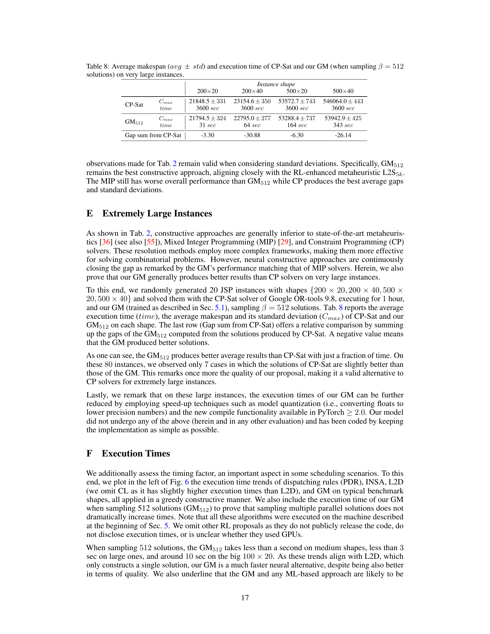
🔼 This table compares the performance of CP-Sat and the proposed Generative Model (GM) on very large JSP instances. It shows the average makespan (Cmax) and its standard deviation, along with the execution time for each solver on four different instance shapes. The ‘Gap sum from CP-Sat’ row indicates the cumulative difference in makespan between the GM and CP-Sat across all instances. Negative values indicate that the GM produced solutions with lower makespans (better performance) than CP-Sat.
read the caption
Table 8: Average makespan (avg ± std) and execution time of CP-Sat and our GM (when sampling β = 512 solutions) on very large instances.
Full paper#
