TL;DR#
Current attention mechanisms in deep learning often use square windows, mixing features from perceptually unrelated image regions and degrading denoising performance. Naive use of superpixels also has limitations, sometimes performing worse than standard attention methods. The main challenge lies in handling the non-rigid boundaries of objects in images, leading to spurious correlations.
This paper introduces Soft Superpixel Neighborhood Attention (SNA), which cleverly interpolates between traditional neighborhood attention and a naive superpixel-based approach. By using superpixel probabilities, SNA effectively re-weights the attention map, addressing the ambiguity and limitations of fixed superpixel assignments. This approach achieves optimal denoising performance under a novel latent superpixel model, outperforming existing methods, and offers a theoretically rigorous framework for incorporating superpixel information into deep learning models.
Key Takeaways#
Why does it matter?#
This paper is important because it proposes a novel attention mechanism that significantly improves image denoising performance. It addresses the limitations of existing methods by incorporating superpixel probabilities, leading to a more robust and accurate approach. This work also opens new avenues for research in attention mechanisms and superpixel-based methods.
Visual Insights#

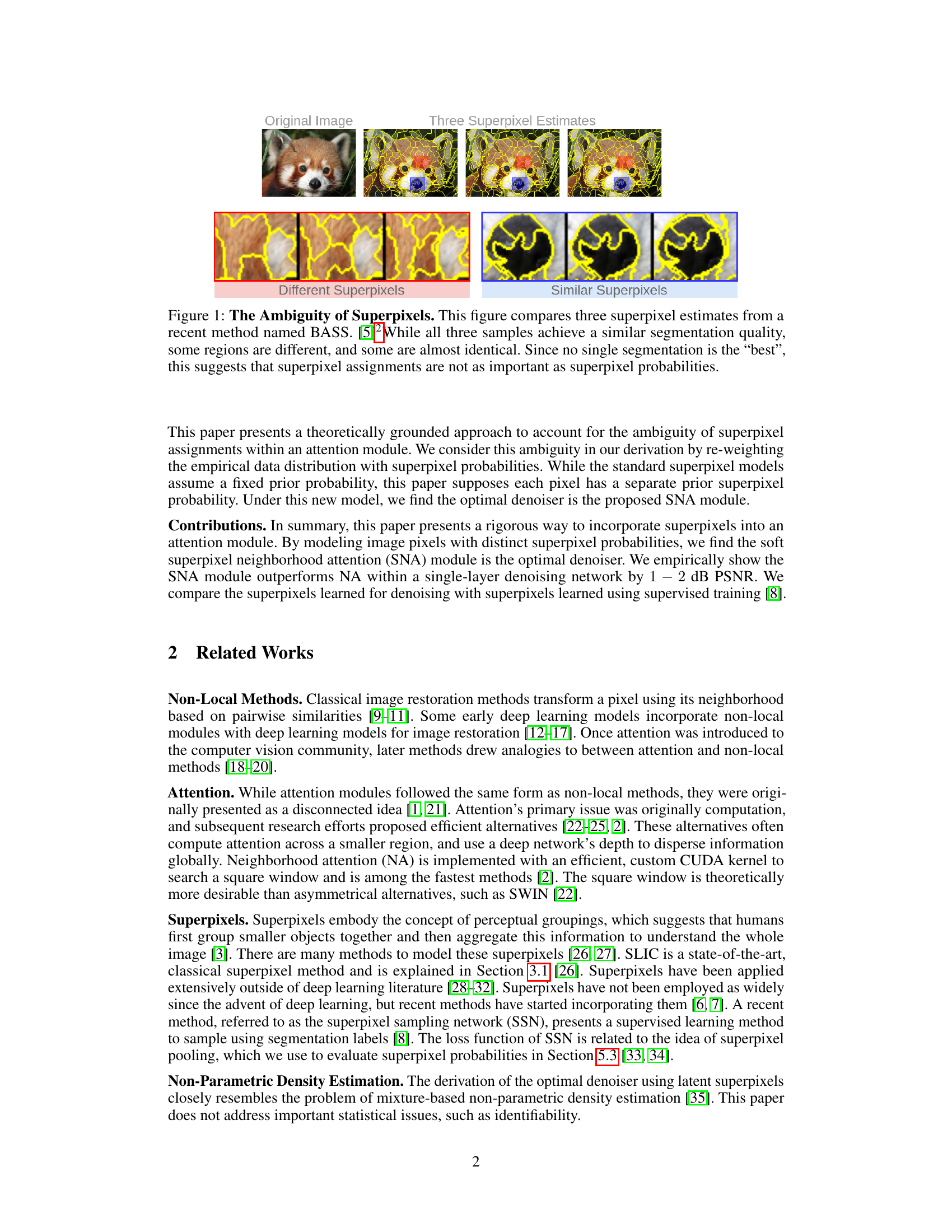
🔼 The figure shows three different superpixel segmentations of the same image produced by the BASS algorithm. Despite the similar overall segmentation quality, there are noticeable differences in the boundaries of the superpixels between the three examples. Some areas show consistent segmentation across all three, while others vary significantly. This illustrates the inherent ambiguity in superpixel segmentation, highlighting the fact that a single, ‘best’ segmentation doesn’t exist. The authors argue that, due to this ambiguity, using superpixel probabilities (the likelihood of a pixel belonging to a given superpixel) is more effective than using hard superpixel assignments (assigning each pixel to only one superpixel).
read the caption
Figure 1: The Ambiguity of Superpixels. This figure compares three superpixel estimates from a recent method named BASS. [5]2While all three samples achieve a similar segmentation quality, some regions are different, and some are almost identical. Since no single segmentation is the 'best', this suggests that superpixel assignments are not as important as superpixel probabilities.
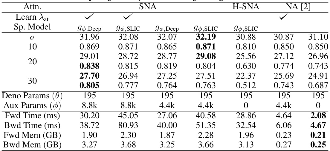
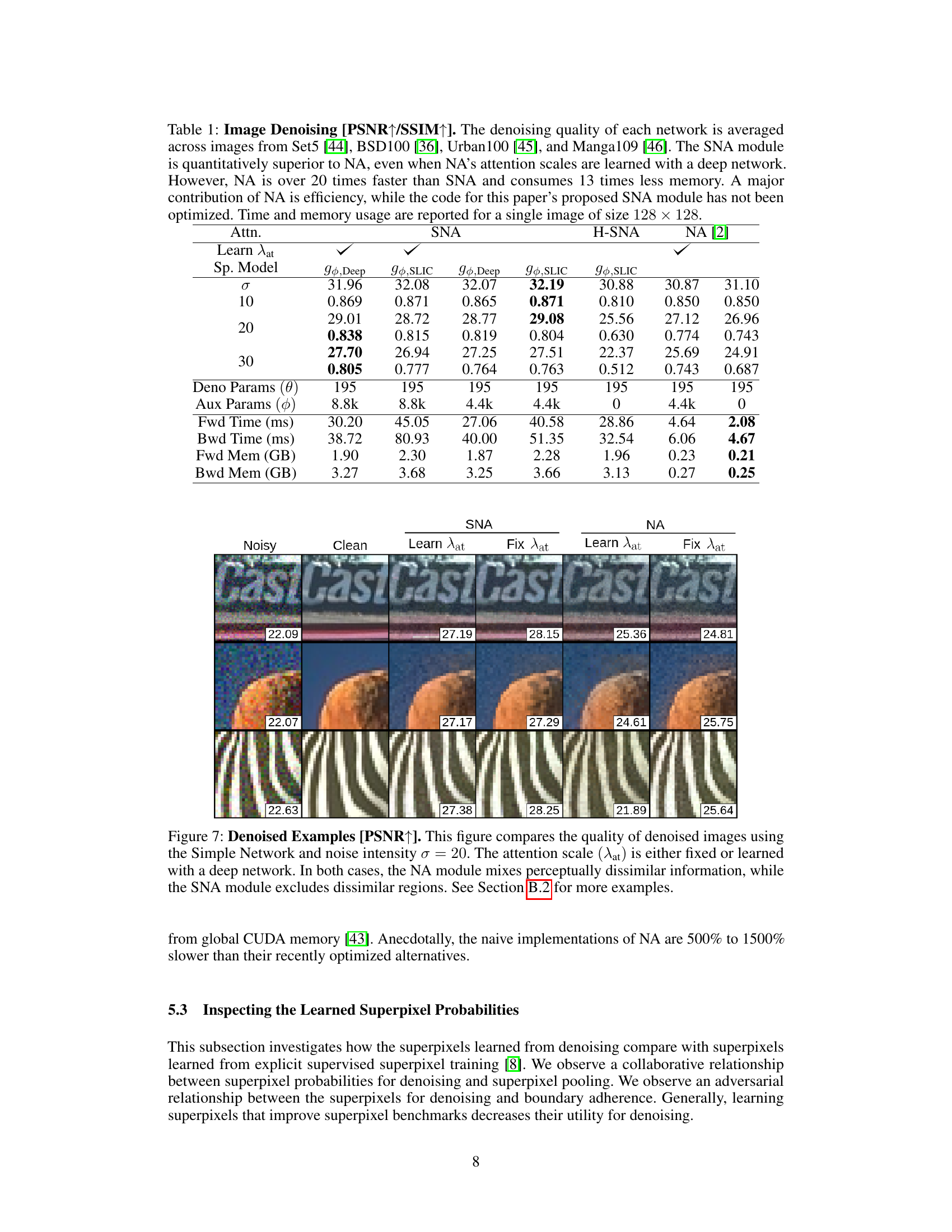
🔼 This table presents quantitative results comparing the performance of different attention mechanisms (SNA, H-SNA, and NA) on Gaussian denoising tasks. It shows Peak Signal-to-Noise Ratio (PSNR) and Structural Similarity Index (SSIM) scores for various noise levels (σ). The table highlights that SNA generally achieves better denoising quality but at a higher computational cost compared to NA. The time and memory usage are also provided for each model.
read the caption
Table 1: Image Denoising [PSNR↑/SSIM↑]. The denoising quality of each network is averaged across images from Set5 [44], BSD100 [36], Urban100 [45], and Manga109 [46]. The SNA module is quantitatively superior to NA, even when NA's attention scales are learned with a deep network. However, NA is over 20 times faster than SNA and consumes 13 times less memory. A major contribution of NA is efficiency, while the code for this paper's proposed SNA module has not been optimized. Time and memory usage are reported for a single image of size 128 × 128.
In-depth insights#
SoftPixel Attention#
SoftPixel Attention, a novel approach in image processing, addresses the limitations of traditional attention mechanisms by incorporating superpixel information. Unlike standard methods that operate on fixed-size square windows, potentially mixing features from unrelated regions, SoftPixel Attention leverages the inherent perceptual groupings of superpixels to create deformable attention windows. This allows the model to focus on coherent regions, improving the quality of feature extraction and reducing the impact of spurious correlations. The method’s ‘softness’ comes from using superpixel probabilities instead of hard assignments, offering a more nuanced and robust approach. This probabilistic approach elegantly handles the inherent ambiguity of superpixel segmentations, making the attention mechanism more resilient to errors in the superpixel estimations. The theoretical analysis demonstrates the optimality of SoftPixel Attention under a latent superpixel model, providing a strong theoretical foundation. The empirical results confirm its superior performance in image denoising compared to standard methods, showcasing the practical benefits of this innovative approach. The integration of learned superpixel probabilities allows the model to seamlessly adapt to various image characteristics, further demonstrating its flexibility and applicability across different scenarios.
Latent Model#
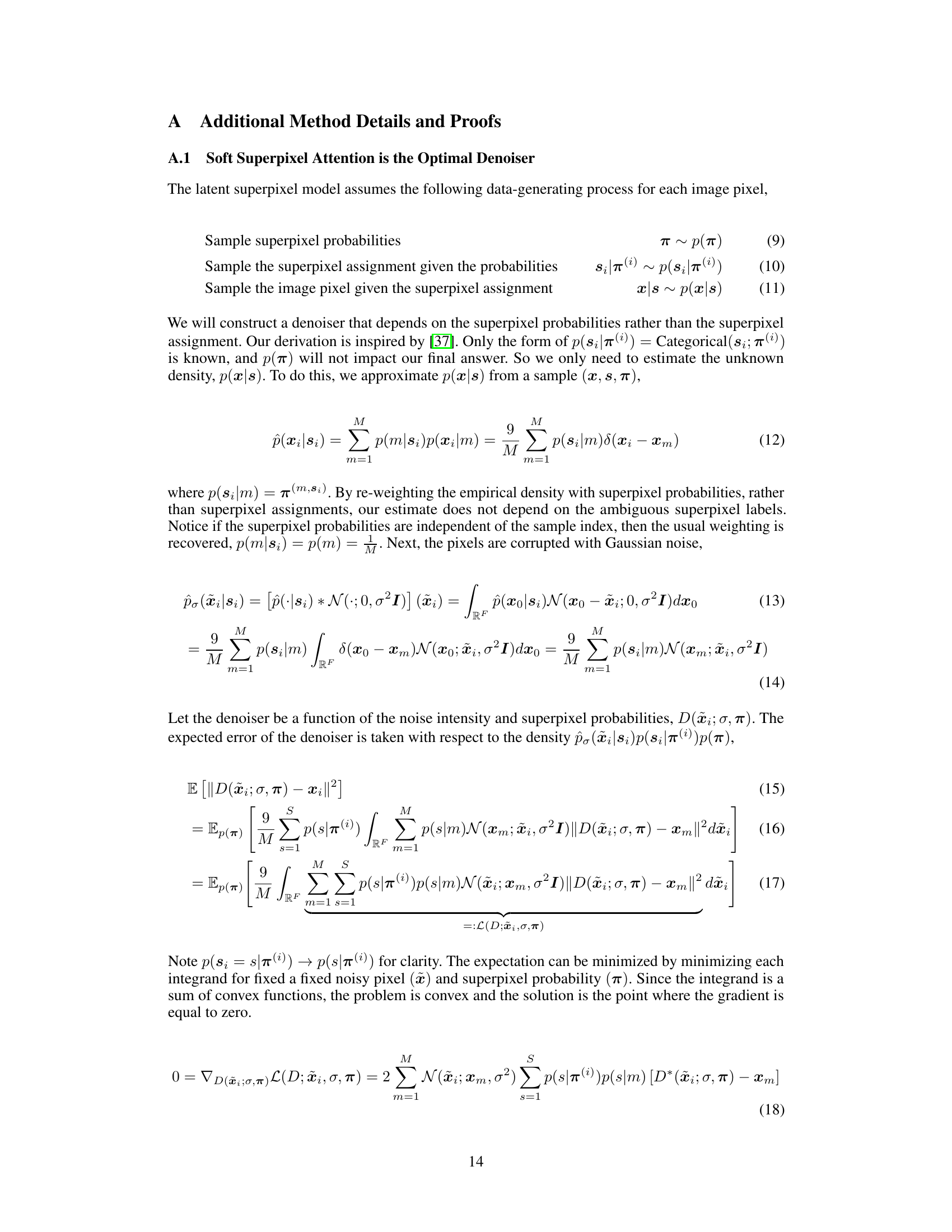
A latent model, in the context of a research paper, likely refers to a statistical model that posits the existence of underlying, unobserved variables (latent variables) that influence the observed data. The core idea is to explain the observed data’s patterns and relationships through these hidden factors, which cannot be directly measured. In this paper, the latent model may focus on the probabilistic nature of superpixel assignments within an image. The model probably assumes that each pixel has an associated probability distribution over possible superpixel memberships, rather than a single hard assignment. This allows for uncertainty and ambiguity in the superpixel segmentation process, which is often inherent in the image data itself. The paper likely uses this latent variable model to derive the optimal denoising function; that is, the model is used to develop a theoretical framework for analyzing the denoising task and deriving an optimal solution. The model likely involves statistical methods, such as Bayesian inference or variational methods, to infer the latent variables from the observed image data. Crucially, this latent model provides a principled way to integrate superpixel information into a denoising model, thereby improving the denoising algorithm’s performance.
Denoising Results#
A comprehensive analysis of denoising results would require examining several key aspects. First, quantitative metrics like PSNR and SSIM are crucial for objectively evaluating the performance of different denoising algorithms. However, these metrics don’t fully capture perceptual quality. Therefore, qualitative assessments through visual inspection of denoised images are equally important to understand how well the algorithms preserve fine details and textures. A critical part of the analysis would be to compare the results against those obtained using different methods. This would involve a thorough comparison of the strengths and weaknesses of each approach in terms of noise reduction effectiveness, computational complexity, and preservation of image features. Additionally, any analysis of denoising results must acknowledge that performance is often highly dependent on the type and level of noise present in the input images. Investigating how the algorithms behave under various noise conditions, and the characteristics of the residual noise after denoising is also necessary. Finally, assessing the robustness of the denoising techniques to various factors is critical, including variations in image content, artifacts, and the level of noise reduction applied.
Superpixel Learning#
Superpixel learning is a crucial aspect of computer vision, aiming to improve image segmentation by grouping similar pixels into meaningful, perceptually coherent units called superpixels. Effective superpixel learning methods are essential for downstream tasks such as object recognition, image retrieval, and denoising. Various strategies exist for learning superpixels, including unsupervised approaches based on clustering algorithms (like SLIC) and supervised methods that leverage labeled datasets to optimize superpixel boundaries. A key challenge is balancing the trade-off between over-segmentation (too many small superpixels, losing important structural information) and under-segmentation (too few large superpixels, failing to capture fine details). The ambiguity inherent in superpixel assignments is a significant issue, especially with irregularly shaped objects where multiple valid segmentations might exist. This necessitates innovative techniques to handle uncertainty in superpixel locations, such as probabilistic superpixel approaches or methods that incorporate superpixel uncertainty directly into attention mechanisms. Recent advancements focus on incorporating deep learning to learn more sophisticated superpixel representations, allowing for adaptability to diverse image types and improved robustness to noise. The future of superpixel learning likely lies in integrating both unsupervised and supervised approaches, taking advantage of the strengths of each to yield highly accurate and robust segmentations.
Computational Cost#
Analyzing the computational cost of the proposed Soft Superpixel Neighborhood Attention (SNA) method reveals a trade-off between accuracy and efficiency. While SNA demonstrably improves denoising performance over traditional Neighborhood Attention (NA), this comes at the cost of increased computational demands. The paper acknowledges that the current SNA implementation is not optimized and that efficiency gains are possible. Future work should focus on optimizing SNA’s implementation, perhaps through algorithmic improvements or hardware acceleration, to mitigate this computational burden. The increased cost primarily stems from the calculation of superpixel probabilities and the re-weighting of the attention map, which are more computationally intensive than NA’s simple neighborhood averaging. The paper provides a quantitative analysis of the computational complexity but does not extensively explore optimization strategies. A detailed comparison of the computation time between SNA and NA should be provided to better illustrate the practical implications of the increased computational cost.
More visual insights#
More on figures

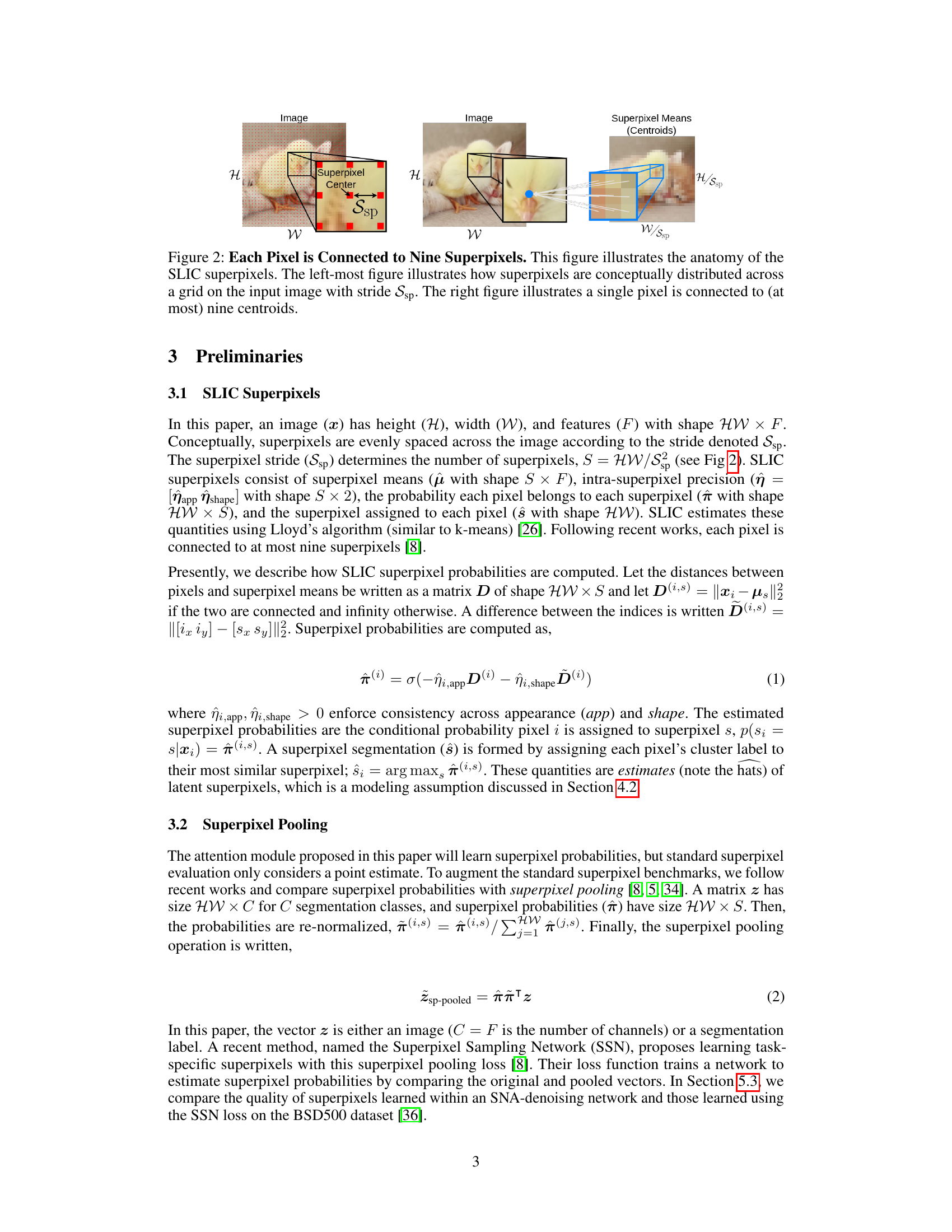
🔼 This figure explains how SLIC superpixels are created and how they relate to individual pixels in an image. The left panel shows a conceptual grid of superpixels overlaid on an image, where each superpixel is a square region with side length Ssp. The middle panel zooms in on a region of the image showing a single pixel, highlighting the nine nearest superpixel centers. The right panel shows those nine superpixel centroids and their associated pixel regions, illustrating how each pixel is connected to multiple superpixels.
read the caption
Figure 2: Each Pixel is Connected to Nine Superpixels. This figure illustrates the anatomy of the SLIC superpixels. The left-most figure illustrates how superpixels are conceptually distributed across a grid on the input image with stride Ssp. The right figure illustrates a single pixel is connected to (at most) nine centroids.

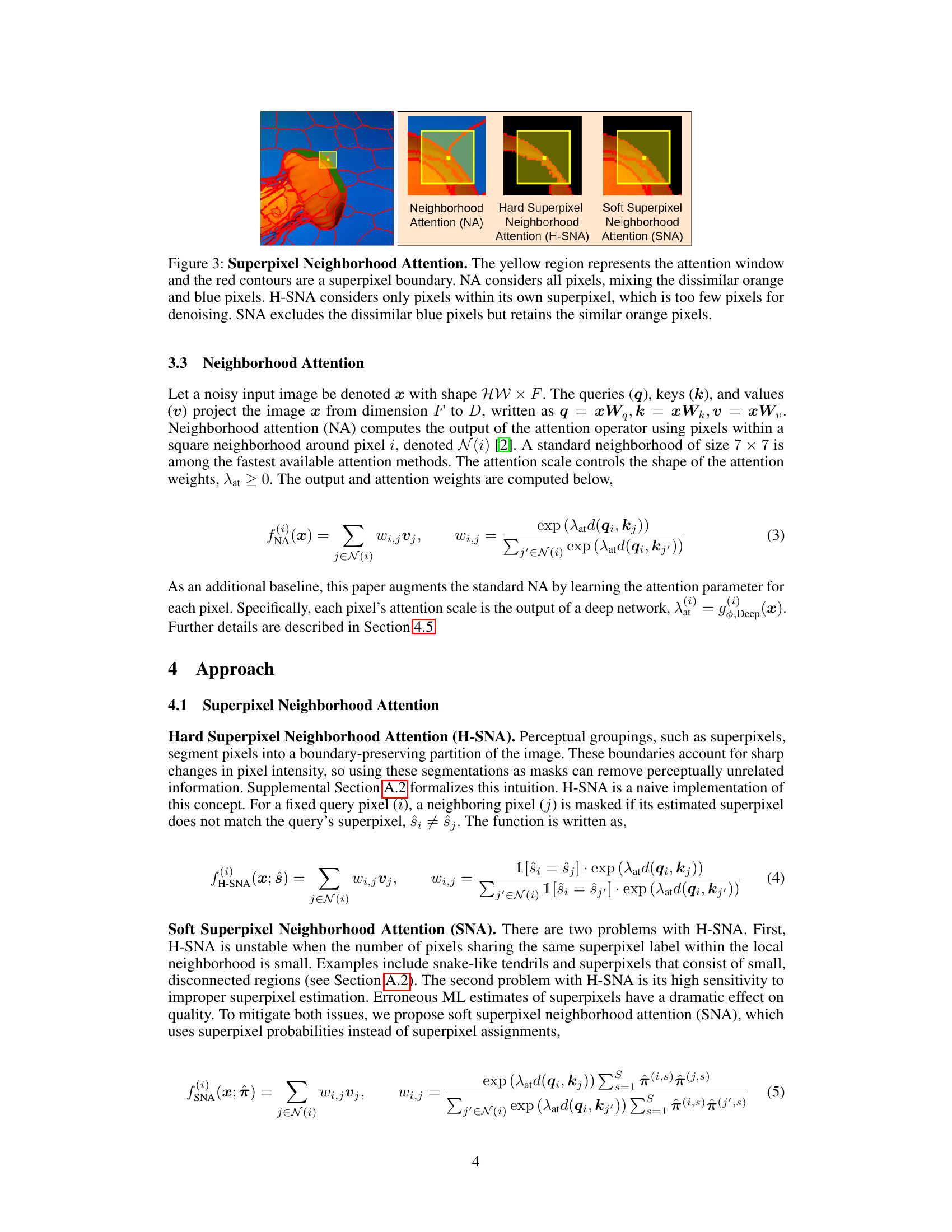
🔼 This figure illustrates the differences between three types of neighborhood attention mechanisms: standard neighborhood attention (NA), hard superpixel neighborhood attention (H-SNA), and soft superpixel neighborhood attention (SNA). NA considers all pixels within a square window, regardless of their perceptual grouping. H-SNA only considers pixels belonging to the same superpixel as the central pixel, potentially missing crucial information. SNA intelligently incorporates superpixel probabilities to selectively weigh pixels, effectively combining the strengths of both NA and H-SNA by including similar pixels and excluding dissimilar ones.
read the caption
Figure 3: Superpixel Neighborhood Attention. The yellow region represents the attention window and the red contours are a superpixel boundary. NA considers all pixels, mixing the dissimilar orange and blue pixels. H-SNA considers only pixels within its own superpixel, which is too few pixels for denoising. SNA excludes the dissimilar blue pixels but retains the similar orange pixels.

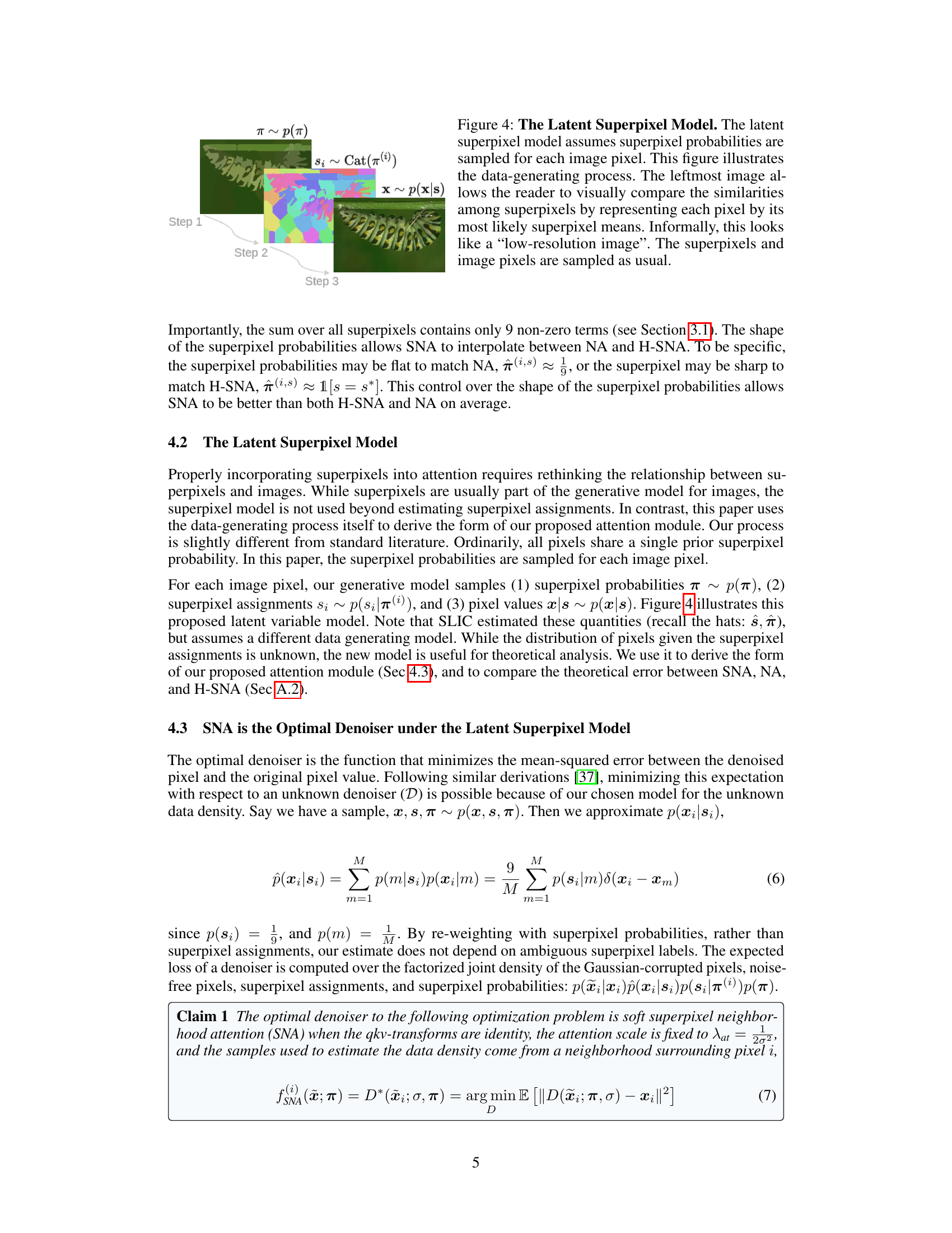
🔼 This figure illustrates the process of generating images according to the latent superpixel model proposed in the paper. First, superpixel probabilities are sampled for each pixel (Step 1). Then, based on these probabilities, a superpixel assignment is made for each pixel (Step 2). Finally, the image pixel values are sampled based on the assigned superpixel (Step 3). The leftmost image shows the superpixel means, creating a low-resolution image representation. The model uses this approach to account for the inherent ambiguity in superpixel assignment.
read the caption
Figure 4: The Latent Superpixel Model. The latent superpixel model assumes superpixel probabilities are sampled for each image pixel. This figure illustrates the data-generating process. The leftmost image allows the reader to visually compare the similarities among superpixels by representing each pixel by its most likely superpixel means. Informally, this looks like a 'low-resolution image'. The superpixels and image pixels are sampled as usual.

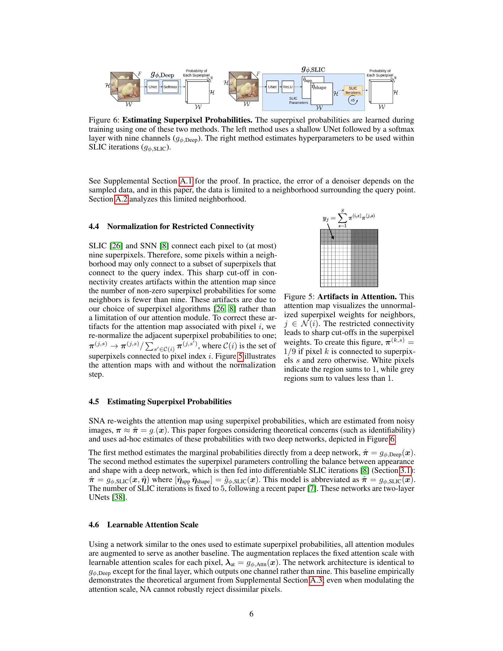
🔼 This figure illustrates two different methods for estimating superpixel probabilities used in the Soft Superpixel Neighborhood Attention (SNA) module. The left side shows a method using a UNet followed by a softmax layer to directly predict probabilities for each superpixel. The right side depicts a method that uses a UNet to estimate hyperparameters for the SLIC superpixel algorithm, which then generates the superpixel probabilities. Both approaches aim to capture the uncertainty in superpixel assignments, providing a soft weighting for attention rather than hard assignments.
read the caption
Figure 6: Estimating Superpixel Probabilities. The superpixel probabilities are learned during training using one of these two methods. The left method uses a shallow UNet followed by a softmax layer with nine channels (gθ,Deep). The right method estimates hyperparameters to be used within SLIC iterations (gθ,SLIC).

🔼 This figure compares three different attention mechanisms: standard neighborhood attention (NA), hard superpixel neighborhood attention (H-SNA), and soft superpixel neighborhood attention (SNA). NA considers all pixels in a square window, leading to the mixing of unrelated features. H-SNA only considers pixels within a single superpixel, which can be insufficient for tasks like denoising. SNA offers a compromise by weighting pixels according to their superpixel probabilities, effectively integrating information from multiple superpixels while focusing on perceptually similar regions.
read the caption
Figure 3: Superpixel Neighborhood Attention. The yellow region represents the attention window and the red contours are a superpixel boundary. NA considers all pixels, mixing the dissimilar orange and blue pixels. H-SNA considers only pixels within its own superpixel, which is too few pixels for denoising. SNA excludes the dissimilar blue pixels but retains the similar orange pixels.
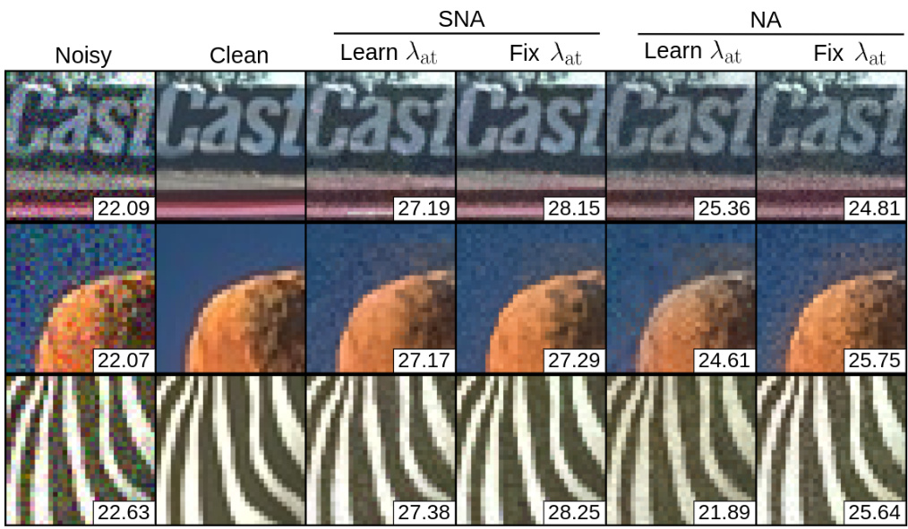
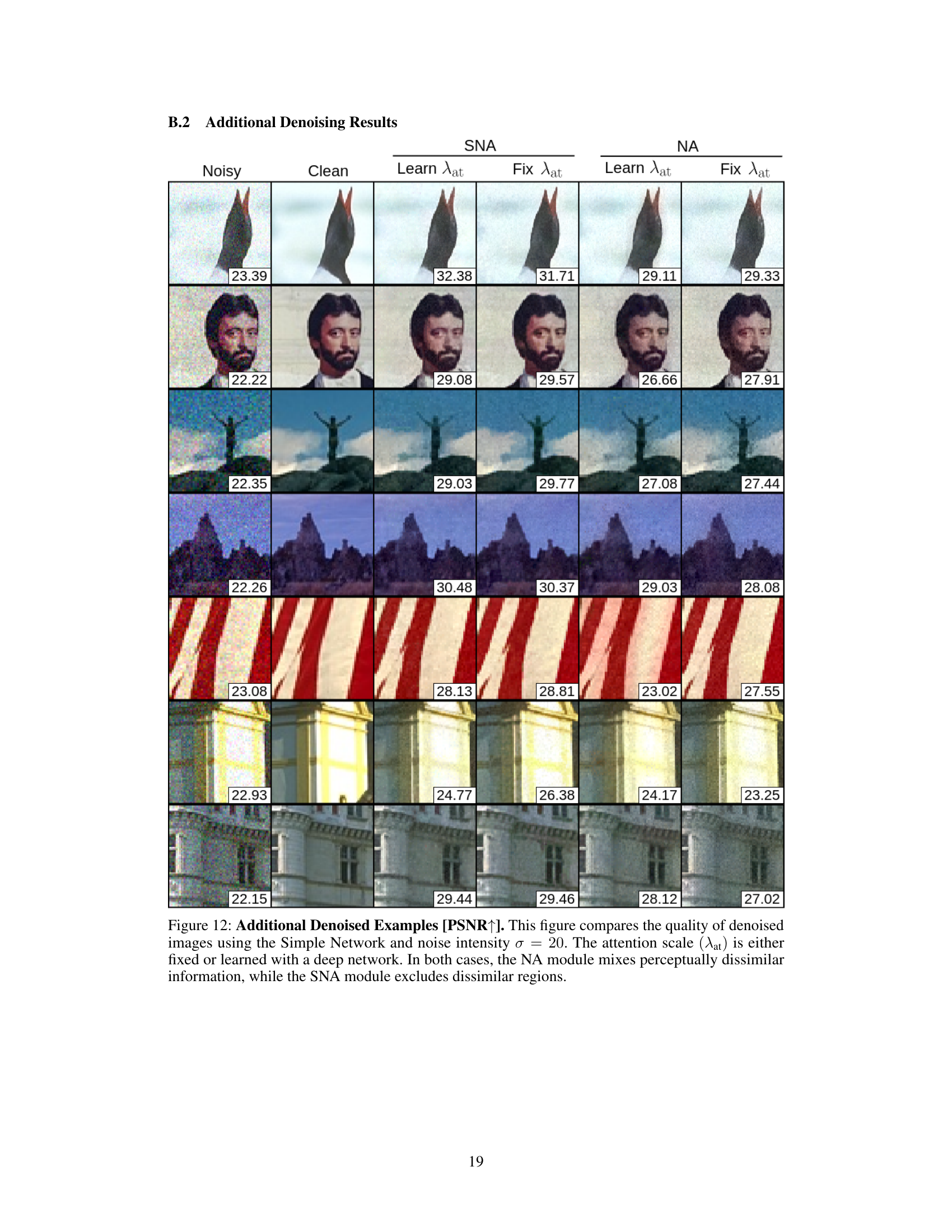
🔼 This figure shows a comparison of denoised images produced by the Simple Network using three different attention methods: standard neighborhood attention (NA), with a fixed or learnable attention scale, and soft superpixel neighborhood attention (SNA), also with fixed or learnable attention scale. The results demonstrate that SNA effectively eliminates perceptually unrelated information, leading to higher quality denoised images, especially evident in the examples where dissimilar image regions are mixed in the NA results. The PSNR values provided quantify this improved quality.
read the caption
Figure 7: Denoised Examples [PSNR↑]. This figure compares the quality of denoised images using the Simple Network and noise intensity σ = 20. The attention scale (λat) is either fixed or learned with a deep network. In both cases, the NA module mixes perceptually dissimilar information, while the SNA module excludes dissimilar regions.

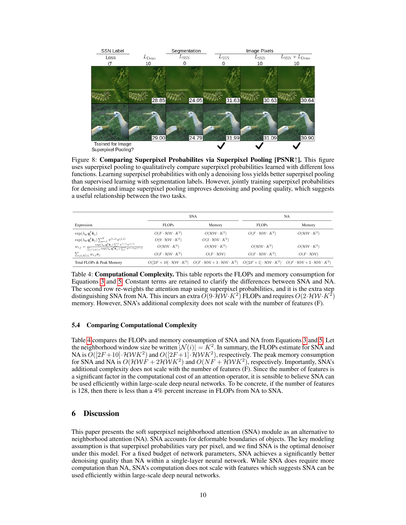
🔼 This figure compares the results of superpixel pooling using superpixel probabilities trained with different loss functions. The top row shows an example image and its superpixel pooled versions. The bottom row shows another example. Each column represents a different training scenario: using only the denoising loss, using only the superpixel loss, using both losses. The PSNR values are shown below each image. The results suggest that training superpixel probabilities with a combination of both denoising and superpixel losses leads to better results than using either loss alone.
read the caption
Figure 8: Comparing Superpixel Probabilites via Superpixel Pooling [PSNR↑]. This figure uses superpixel pooling to qualitatively compare superpixel probabilities learned with different loss functions. Learning superpixel probabilities with only a denoising loss yields better superpixel pooling than supervised learning with segmentation labels. However, jointly training superpixel probabilities for denoising and image superpixel pooling improves denoising and pooling quality, which suggests a useful relationship between the two tasks.

🔼 This figure shows the effect of increasing neighborhood size on denoising performance for three different noise levels (σ = 10, 20, 30). As the neighborhood size grows, the variance decreases (leading to better denoising), but the bias increases (introducing errors). This is a bias-variance tradeoff, and the optimal neighborhood size increases as noise increases. The Hard Superpixel Neighborhood Attention (H-SNA) method, having a bias close to zero, shows improved denoising performance with increasing neighborhood size.
read the caption
Figure 9: Neighborhood Window Size. Increasing the neighborhood window size includes more samples to decrease the variance but also adds bias since the noisy samples can be weighted improperly. This bias-variance trade-off is illustrated by the increasing optimal window size as the noise intensity increases. Since the bias of H-SNA is nearly zero, the increasing neighborhood size only increases the denoising quality within the selected grid.
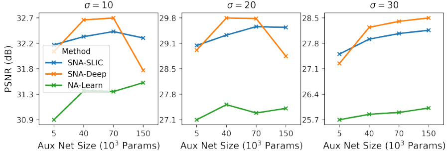
🔼 This ablation study investigates the effect of varying the size of the auxiliary network on denoising performance. The plot shows PSNR values for different noise levels (σ = 10, 20, 30) as a function of the number of parameters in the auxiliary network. The results suggest that larger auxiliary networks generally lead to better denoising performance, although there’s a possible indication of overfitting at the largest network size tested.
read the caption
Figure 10: Number of Auxiliary Parameters. This ablation experiment expands the size of the auxiliary network by increasing the number of UNet channels. The x-axis plots the number of parameters in the auxiliary network (||). The y-axis plots the PSNR of several denoiser networks. Generally, more parameters improve the denoising quality. The drop in denoising quality for the final network may be due to under-training.
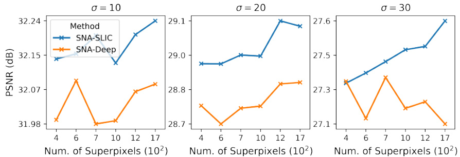
🔼 This figure shows the effect of the number of superpixels on denoising performance for different noise levels (σ = 10, 20, 30). The results indicate that while increasing the number of superpixels generally improves denoising quality, this effect is more pronounced at higher noise levels. At low noise levels, the number of superpixels appears less critical. Additionally, using the SLIC algorithm directly to generate superpixels produces slightly better results than learning them from a neural network.
read the caption
Figure 11: Number of Superpixels. The number of superpixels has a limited effect on the denoising quality when compared with other hyperparameters. Generally, increasing the number of superpixels increases the denoising quality. When the noise is low (σ = 10) the number of superpixels seems irrelevant. As the noise increases, the benefit of more superpixels becomes more apparent. Generally, using explicit SLIC iterations is more effective than predicting superpixel probabilities directly.
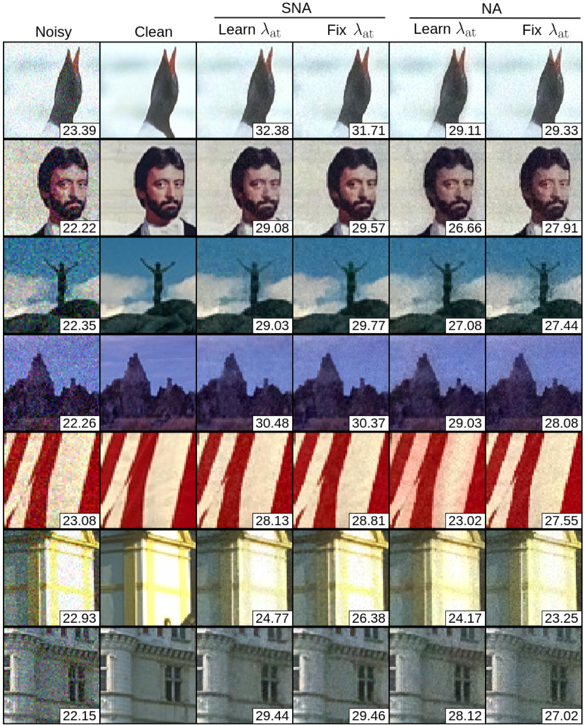
🔼 This figure compares the denoising results of the proposed SNA and standard NA methods on several images with noise intensity σ = 20. It shows that SNA outperforms NA in terms of visual quality and PSNR values by excluding dissimilar regions and preserving similar regions within the attention windows, while NA mixes perceptually unrelated pixels leading to a decrease in the overall quality.
read the caption
Figure 7: Denoised Examples [PSNR↑]. This figure compares the quality of denoised images using the Simple Network and noise intensity σ = 20. The attention scale (λat) is either fixed or learned with a deep network. In both cases, the NA module mixes perceptually dissimilar information, while the SNA module excludes dissimilar regions.
More on tables

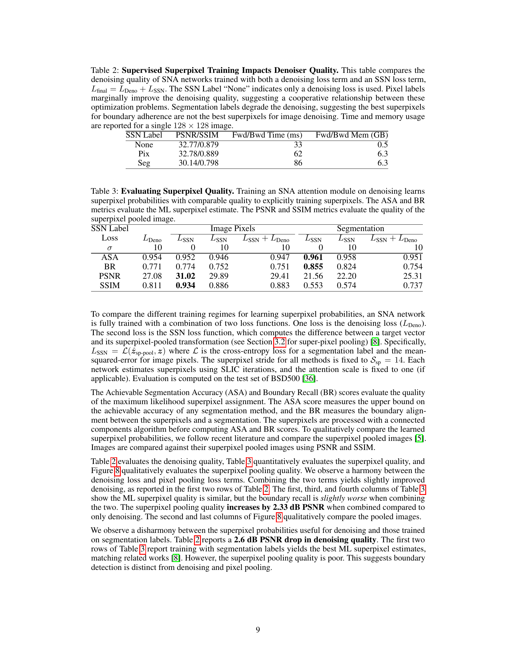
🔼 This table shows the results of training SNA networks with different loss functions. It compares denoising performance (PSNR/SSIM) when only using a denoising loss, when adding a pixel-level supervised loss, and when adding a segmentation-level supervised loss. The results show that adding a pixel-level loss slightly improves denoising, while adding a segmentation-level loss significantly degrades performance, suggesting a trade-off between boundary accuracy and denoising quality. Computational cost (time and memory usage) is also provided.
read the caption
Table 2: Supervised Superpixel Training Impacts Denoiser Quality. This table compares the denoising quality of SNA networks trained with both a denoising loss term and an SSN loss term, Lfinal = LDeno + Lssn. The SSN Label “None” indicates only a denoising loss is used. Pixel labels marginally improve the denoising quality, suggesting a cooperative relationship between these optimization problems. Segmentation labels degrade the denoising, suggesting the best superpixels for boundary adherence are not the best superpixels for image denoising. Time and memory usage are reported for a single 128 × 128 image.

🔼 This table compares the quality of superpixels learned by training a soft superpixel neighborhood attention (SNA) module for image denoising with the quality of superpixels learned using a supervised training method. It evaluates both the accuracy of the maximum likelihood superpixel estimate (using Achievable Segmentation Accuracy (ASA) and Boundary Recall (BR)) and the quality of the resulting image after superpixel pooling (using Peak Signal-to-Noise Ratio (PSNR) and Structural Similarity Index (SSIM)). The comparison helps to determine whether learning superpixels for denoising produces superpixels that are similarly effective for other tasks (like supervised superpixel segmentation).
read the caption
Table 3: Evaluating Superpixel Quality. Training an SNA attention module on denoising learns superpixel probabilities with comparable quality to explicitly training superpixels. The ASA and BR metrics evaluate the ML superpixel estimate. The PSNR and SSIM metrics evaluate the quality of the superpixel pooled image.

🔼 This table compares the denoising performance of different attention mechanisms (SNA and NA) under various conditions (learning attention scale or not, using SLIC superpixels or not) across four benchmark image datasets. It shows that SNA generally outperforms NA in terms of PSNR and SSIM, although NA is significantly faster and more memory-efficient.
read the caption
Table 1: Image Denoising [PSNR↑/SSIM↑]. The denoising quality of each network is averaged across images from Set5 [44], BSD100 [36], Urban100 [45], and Manga109 [46]. The SNA module is quantitatively superior to NA, even when NA's attention scales are learned with a deep network. However, NA is over 20 times faster than SNA and consumes 13 times less memory. A major contribution of NA is efficiency, while the code for this paper's proposed SNA module has not been optimized. Time and memory usage are reported for a single image of size 128 × 128.

🔼 This table presents a quantitative comparison of different attention mechanisms for image denoising. It shows the Peak Signal-to-Noise Ratio (PSNR) and Structural Similarity Index (SSIM) scores for various noise levels (σ). The results demonstrate that the proposed Soft Superpixel Neighborhood Attention (SNA) significantly outperforms standard Neighborhood Attention (NA), especially at higher noise levels. However, it highlights the computational cost and memory usage of SNA, emphasizing the efficiency advantage of NA.
read the caption
Table 1: Image Denoising [PSNR↑/SSIM↑]. The denoising quality of each network is averaged across images from Set5 [44], BSD100 [36], Urban100 [45], and Manga109 [46]. The SNA module is quantitatively superior to NA, even when NA's attention scales are learned with a deep network. However, NA is over 20 times faster than SNA and consumes 13 times less memory. A major contribution of NA is efficiency, while the code for this paper's proposed SNA module has not been optimized. Time and memory usage are reported for a single image of size 128 × 128.
Full paper#

