↗ OpenReview ↗ NeurIPS Homepage ↗ Chat
TL;DR#
Understanding the complex dynamics of neural systems is a major challenge. Traditional methods often struggle with noisy data and high dimensionality, limiting interpretability. Existing models that do incorporate stochasticity often lack analytical tractability, hindering analysis of underlying dynamics. This makes it difficult to build accurate and insightful models of neural activity.
This paper introduces a new method to address these limitations. By fitting stochastic low-rank recurrent neural networks (RNNs) using variational sequential Monte Carlo, the researchers developed a technique that is both interpretable and fits neural data well. This new approach also includes a method for efficiently determining all fixed points in polynomial time, a considerable improvement over existing exponential time approaches. The method’s effectiveness was demonstrated on several real-world datasets, outperforming current state-of-the-art methods in terms of lower dimensional latent dynamics.
Key Takeaways#
Why does it matter?#
This paper is crucial for researchers in computational neuroscience and machine learning. It offers a novel method to infer interpretable stochastic dynamical systems from noisy neural data, advancing our understanding of brain function and providing valuable tools for model development. The efficient fixed-point identification technique significantly improves the tractability of complex model analysis. The work opens avenues for studying neural variability and complex brain dynamics using sophisticated modeling techniques.
Visual Insights#

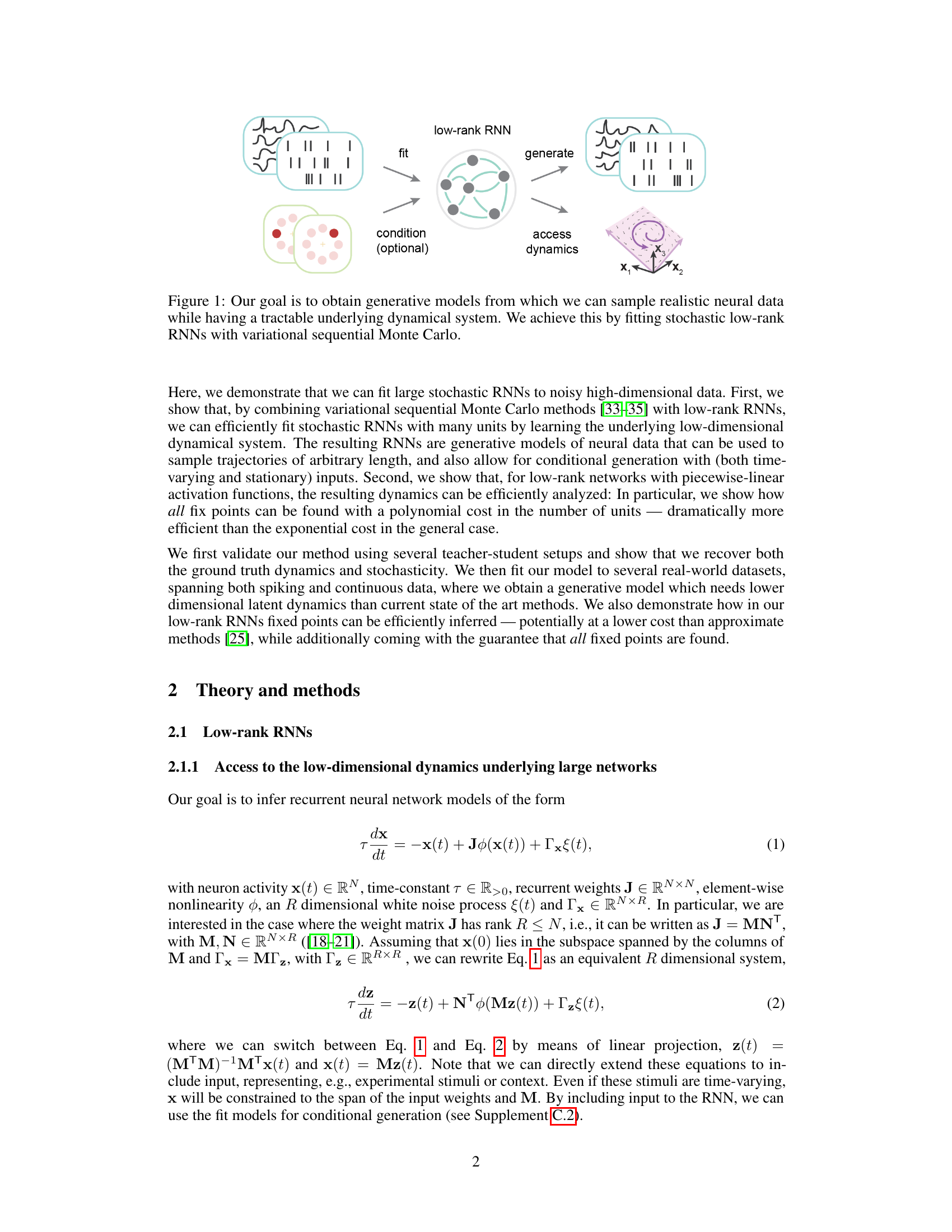
This figure illustrates the overall workflow of the proposed method. The goal is to build generative models of neural data that are both realistic and have a simple, understandable underlying dynamical system. This is accomplished by fitting stochastic low-rank recurrent neural networks (RNNs) to high-dimensional, noisy neural data using variational sequential Monte Carlo methods. The figure shows how the method takes noisy neural data as input and fits a low-rank RNN model to it. Then, using this model, one can generate new samples of realistic neural data, access and analyze the low-dimensional latent dynamics, and optionally, use conditional generation by providing external context or stimuli.

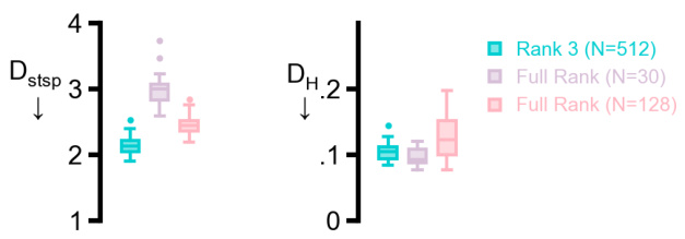
This table compares the performance of the proposed SMC method with the state-of-the-art GTF method in terms of model dimensionality and reconstruction accuracy. Lower values of Dstsp and DH indicate better reconstruction quality, while ‘dim’ represents the dimensionality of the latent dynamical system and |θ| represents the number of trainable parameters. The results show that the SMC method achieves similar reconstruction accuracy to GTF but with significantly lower dimensionality (3 vs 16).
In-depth insights#
Stochastic RNNs#
Stochastic recurrent neural networks (RNNs) represent a powerful class of models for capturing temporal dynamics in data, particularly where inherent randomness or noise plays a significant role. Unlike deterministic RNNs, stochastic RNNs incorporate probabilistic transitions, meaning the next state of the network is not solely determined by the current state but also influenced by a random element. This randomness is crucial in modeling real-world systems where unpredictable events occur. Variational methods, such as variational sequential Monte Carlo (SMC), provide effective means to infer the parameters of stochastic RNNs from noisy data. SMC techniques allow for the estimation of complex probability distributions in the high-dimensional state space of the RNN, facilitating model fitting and parameter learning. Further, the introduction of stochasticity often reduces the need for high-dimensional deterministic models by allowing for more compact representations of complex temporal behaviors. The trade-off between the accuracy of model fitting and model interpretability is managed by the chosen model architecture (e.g., low-rank RNNs), which further enhances the effectiveness of stochastic RNNs in various applications.
Variational Inference#
Variational inference (VI) is a powerful approximate inference technique, particularly valuable when dealing with complex probability distributions intractable via exact methods. Its core idea is to approximate a target distribution (often a posterior in Bayesian settings) with a simpler, tractable distribution from a chosen family. This approximating distribution is optimized to be as close as possible to the target, typically measured by minimizing the Kullback-Leibler (KL) divergence. The method’s effectiveness hinges on the choice of the approximating family; a flexible family allows for tighter approximations but increases computational cost. Common choices include Gaussian distributions (mean-field VI) or more sophisticated families like variational autoencoders (VAEs). The optimization process often involves iterative updates to the parameters of the approximating distribution, employing gradient-based methods. While VI offers significant advantages in scalability and tractability, it introduces bias, and the quality of the approximation depends heavily on the choice of the approximating family and the algorithm used. Careful consideration of these aspects is crucial to ensure reliable inference.
Low-rank Dynamics#
Low-rank dynamics in neural systems offer a powerful framework for understanding high-dimensional neural activity through a lens of reduced dimensionality. The core idea is that despite the complexity of neural interactions, the underlying dynamics might be governed by a lower-dimensional latent space. This simplification significantly enhances interpretability and facilitates the development of tractable computational models. By identifying these lower-dimensional representations, we gain a deeper understanding of how complex neural computations are executed, reducing the analytical complexity inherent in handling the full dimensionality of the neural population. This approach also leads to efficient inference methods that can effectively extract these low-rank representations from noisy neural data. The practical implications are significant, allowing researchers to develop generative models that accurately capture the observed variability in neural recordings. However, it’s crucial to consider the limitations of this approach, as the assumption of low-rank structure might not always hold true for all neural systems and tasks. Careful validation and consideration of alternative models are necessary to ensure the reliability and generalizability of findings based on low-rank dynamics. The success of this approach hinges on the ability to appropriately select and extract these low-dimensional features from the observed data.
Fixed Point Analysis#
Analyzing fixed points in recurrent neural networks (RNNs) offers crucial insights into their dynamics and computational capabilities. Low-rank RNNs, in particular, are attractive due to their tractability, making fixed point analysis computationally feasible. For networks with piecewise-linear activation functions, such as ReLU, identifying fixed points becomes particularly efficient. Instead of an exponential cost associated with traditional methods, polynomial-time algorithms become possible, significantly reducing computational complexity. This advantage stems from the ability to efficiently partition the state space into linear regions, enabling analysis within those regions. The identification of all fixed points allows for a comprehensive understanding of the network’s attractor landscape and its behavior in the absence of external input. Analyzing fixed points is crucial to interpreting the RNN as a dynamical system, as fixed points correspond to stable states or steady-state behavior. The analytical tractability of finding fixed points for these specialized low-rank, piecewise-linear RNNs significantly enhances the interpretability of these models in neuroscience and other applications.
Future Directions#
Future research could explore non-Gaussian noise processes in the recurrent dynamics, enhancing biological realism. Investigating interactions between LFP and spike phases using multi-modal setups or multi-region analyses is crucial for understanding hippocampal function. Improving scalability for higher-dimensional datasets is key to expanding applications. Exploring different nonlinear activation functions beyond piecewise-linear may enhance model expressiveness and uncover more complex dynamics. Finally, a rigorous comparison with state-space models and other advanced methods is needed to solidify the proposed approach’s strengths and limitations. Addressing these points will greatly advance the field of neural data analysis and brain dynamics modeling.
More visual insights#
More on figures
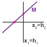
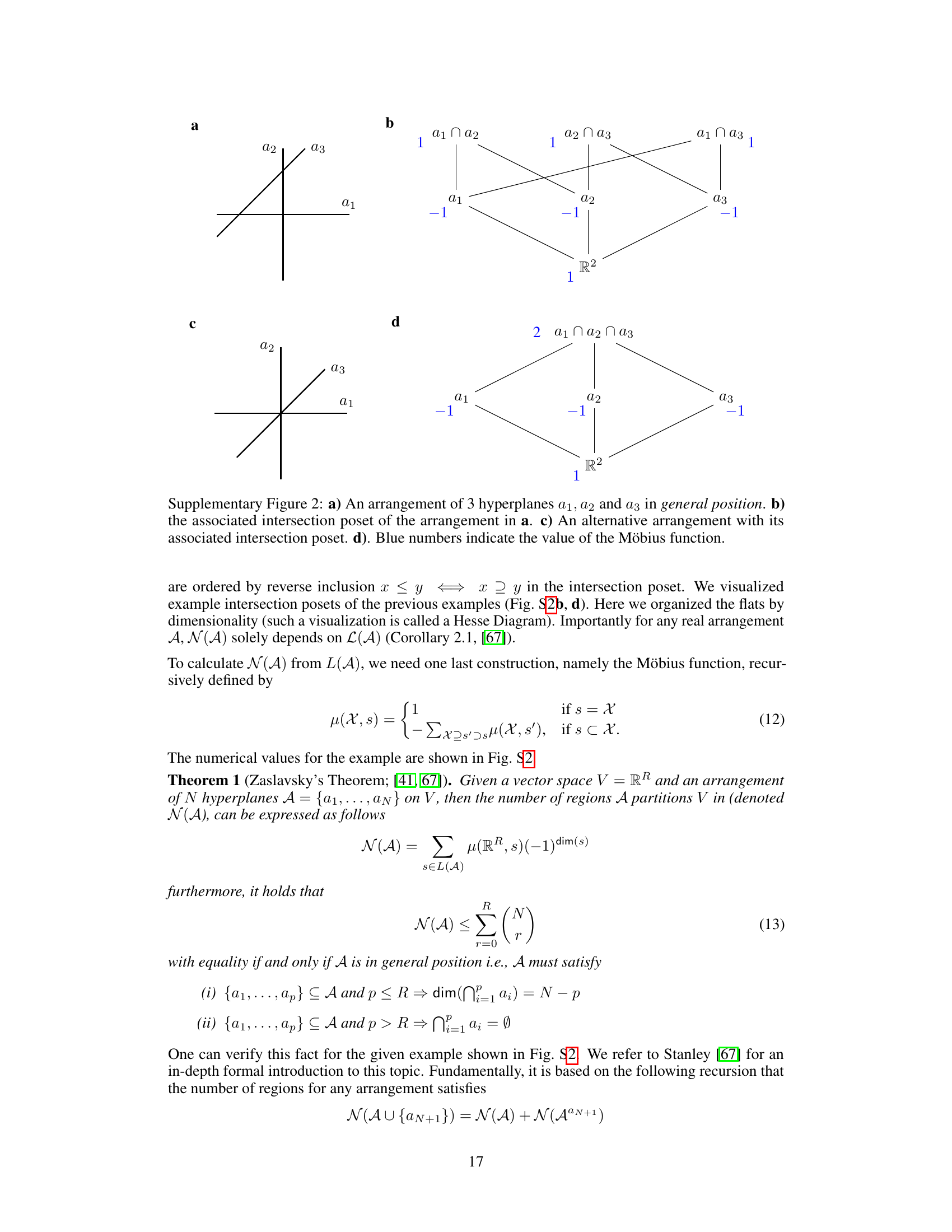
This figure is a sketch to illustrate the proof of Proposition 1, which states that the computational cost of finding all fixed points in a low-rank RNN with piecewise-linear activation functions is polynomial rather than exponential in the number of units. The figure shows a two-dimensional phase space divided into four regions by two hyperplanes. The proof leverages Zaslavsky’s Theorem on hyperplane arrangements to show that if the dynamics are constrained to a lower-dimensional subspace (as they are in low-rank systems), the number of regions that need to be considered is significantly reduced, leading to a polynomial computational complexity.

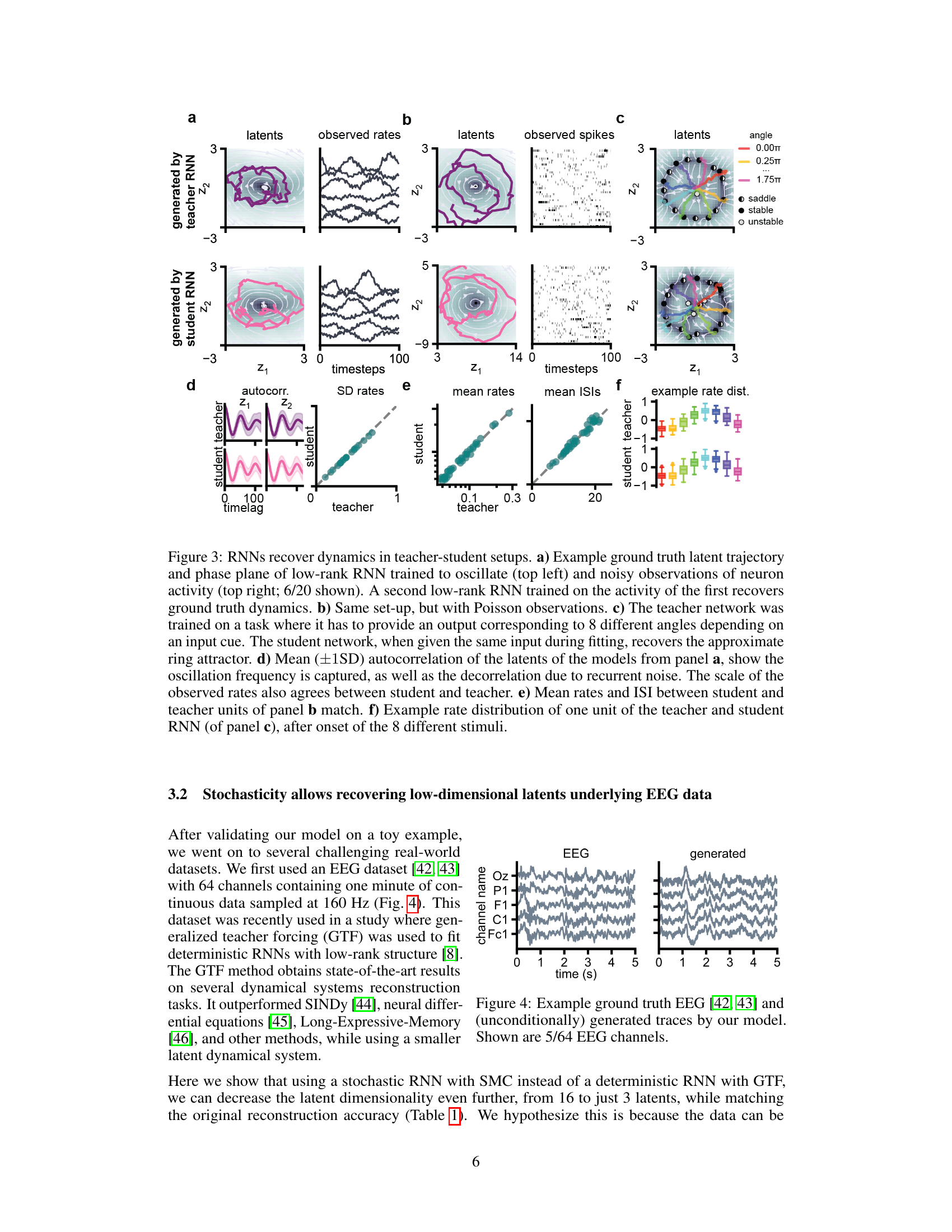
This figure demonstrates the ability of the proposed method to recover the ground truth dynamics and stochasticity from noisy high-dimensional data. It shows the results of three teacher-student experiments, where a ’teacher’ RNN generates data, and a ‘student’ RNN is trained on this data. Panel (a) and (b) demonstrates the recovery of continuous and spiking data, respectively, while panel (c) demonstrates recovery when an input cue is included. The remaining panels (d)-(f) show additional quantitative analyses, demonstrating that the student RNN captures the underlying dynamics, stochasticity, and response properties of the teacher RNN.
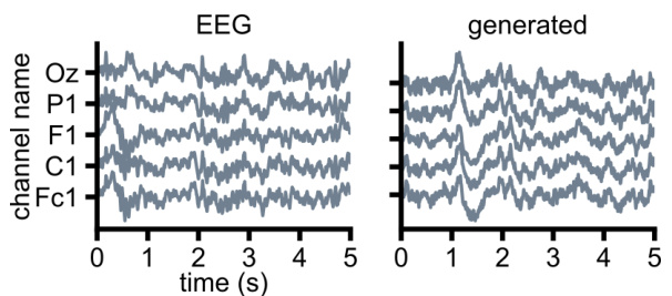
This figure demonstrates the ability of the proposed stochastic low-rank RNN model to generate realistic EEG data. The left panel shows example traces from real EEG data recorded from 5 out of 64 channels. The right panel shows traces generated by the model. The close visual similarity between the real and generated data highlights the model’s capacity to capture the complex temporal dynamics of EEG signals.

This figure demonstrates the ability of the proposed method to recover ground truth dynamics and stochasticity from noisy data. Panel (a) shows a teacher-student setup with Gaussian noise, (b) with Poisson noise, and (c) with a task involving an input cue. Panels (d)-(f) provide additional analyses of the results, including autocorrelation of latent variables, mean firing rates and ISIs, and example rate distributions.
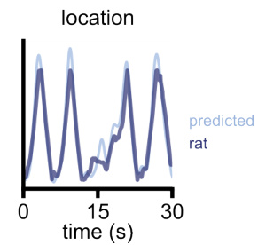
This figure shows that the posterior latents obtained from a rank-4 RNN trained solely on spiking activity from rat hippocampus can be used to predict the rat’s position on a linear track. The model accurately reconstructs the distribution of spikes and exhibits oscillations in its latents. The posterior latents also show a strong relationship with the rat’s position, indicating that the model captures the underlying dynamics of the spiking data and successfully integrates this information with the rat’s position.
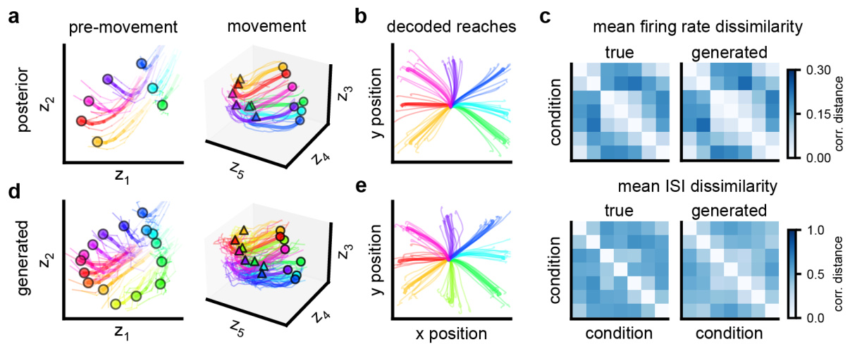
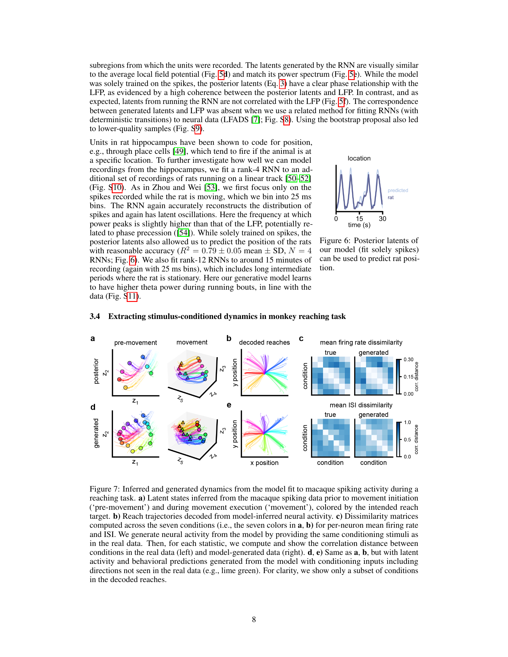
This figure shows the results of applying the proposed method to macaque spiking data during a reaching task. Panel (a) displays inferred latent states before and during movement, colored by reach target. Panel (b) shows decoded reach trajectories from the model. Panel (c) compares dissimilarity matrices of firing rates and inter-spike intervals (ISIs) between conditions in real and generated data. Panels (d) and (e) repeat the analysis in (a) and (b) but using generated data from the model conditioned on unseen inputs, demonstrating generalization ability.

This figure compares the performance of three methods for finding fixed points in a piecewise-linear RNN: an analytic method, an approximate method, and a combined method that uses the analytic method to constrain the search space of the approximate method. The x-axis represents the number of matrix inverses computed, and the y-axis represents the number of fixed points found. The analytic method consistently finds all 17 fixed points, while the approximate method finds fewer fixed points and its performance varies across different runs. The combined method improves upon the approximate method by using the analytic method to reduce the search space, but it still finds fewer fixed points than the analytic method.

This figure is a sketch to help understand the proof of Proposition 1. It illustrates how the computational cost of finding all fixed points in piecewise-linear low-rank RNNs can be reduced from exponential to polynomial in the number of units. In a high-dimensional network with N units, the phase space is divided into 2N regions. However, if the dynamics are constrained to a lower-dimensional subspace of rank R, spanned by the columns of the matrix M, the number of regions considered is greatly reduced. Each hyperplane (pink points) determined by a unit partitions the subspace. The number of such regions is polynomial in N for a fixed R, as shown by the application of Zaslavsky’s theorem. This implies that finding all fixed points can be done efficiently, contrary to the naive approach that has an exponential complexity.
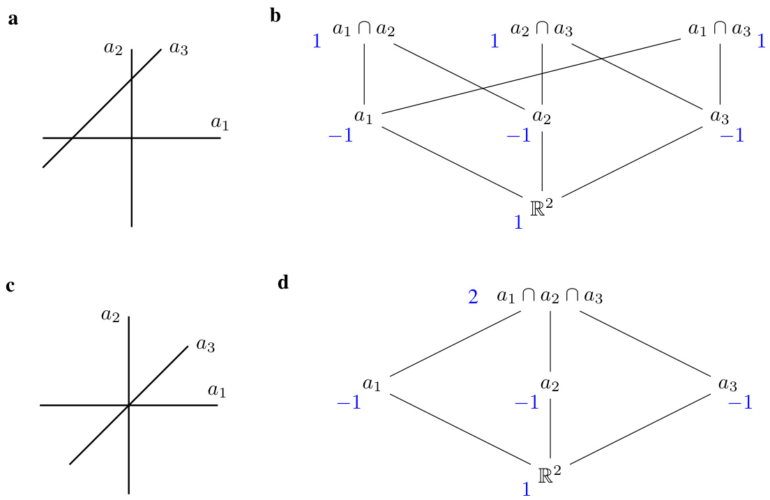
This figure is a sketch to help understand the proof of Proposition 1. It illustrates how, for low-rank networks with piecewise-linear activation functions, the cost of finding all fixed points is polynomial rather than exponential in the number of units. The figure shows how the activation functions partition the phase space into linear regions. The key idea is that, because the dynamics are low-rank, only a subset of these linear regions are accessible, drastically reducing the number of calculations needed to find all fixed points.

This figure demonstrates the ability of the proposed method to recover ground truth dynamics from noisy data. It presents results from several teacher-student experiments where a low-rank RNN (the student) was trained to mimic the behavior of a teacher RNN with known dynamics and added noise. Panel (a) shows results for continuous data and (b) for spiking data; (c) demonstrates the method’s ability to learn dynamics in the presence of time-varying input. Panels (d), (e), and (f) provide additional statistical analyses to support the claim that the student RNN effectively replicates the teacher RNN’s dynamics, stochasticity, and response to stimuli.

This figure demonstrates the ability of low-rank RNNs to recover ground truth dynamics from noisy data in teacher-student experiments. Panels (a) and (b) show that the student RNN successfully recovers the latent dynamics and noise level of the teacher RNN, for both continuous and Poisson observations. Panel (c) showcases the ability of the model to recover a ring attractor representing a task involving the processing of angular cues. Panels (d)-(f) provide further validation by demonstrating matches in autocorrelations of latents, mean firing rates, and inter-spike interval distributions, respectively.

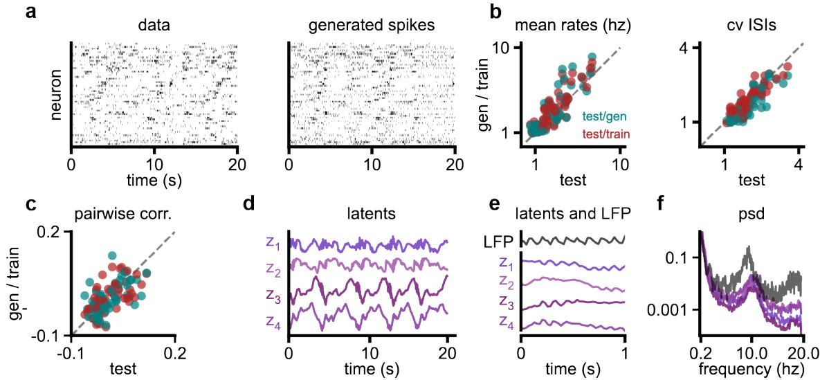
This figure demonstrates the ability of the proposed stochastic low-rank RNN model to accurately capture the statistical properties of real-world spiking neural data. Panel (a) shows the model’s ability to generate realistic spike trains resembling recordings from rat hippocampus. Panels (b-c) quantitatively demonstrate the accuracy of the model by comparing single-neuron and population-level statistics of generated and held-out test data. The remaining panels (d-f) focus on the model’s ability to recover low-dimensional latent dynamics that are strongly related to the local field potential (LFP), demonstrating its capacity to uncover meaningful underlying brain dynamics.

This figure shows the results of teacher-student experiments where a low-rank RNN (teacher) is trained to generate oscillatory activity or perform a task involving angle recognition based on input stimuli, and another low-rank RNN (student) is trained on the generated data to recover the underlying dynamics. Panels a and b demonstrate the recovery of continuous and Poisson spiking data respectively. Panel c demonstrates recovery of dynamics for a task involving angle recognition. Panels d, e, and f provide supplementary statistics such as autocorrelation of latents, mean rates and inter-spike intervals, and example rate distribution to support the claim of successful recovery of dynamics and stochasticity.
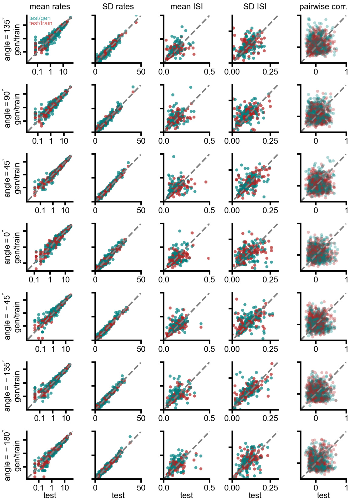
This figure demonstrates the ability of the proposed method to recover the ground truth dynamics and stochasticity of a teacher RNN from noisy observations. It shows results for three different teacher-student setups: one with continuous Gaussian observations, one with Poisson observations, and one with a task involving angle-dependent stimuli. The figure demonstrates that the student RNNs accurately recover the latent dynamics of the teacher RNNs, including the level of stochasticity, oscillation frequency, and response to external stimuli. This is further validated by comparing autocorrelations, mean firing rates, inter-spike intervals, and example rate distributions between the teacher and student models across different conditions.

This figure demonstrates the ability of the proposed method to recover the ground truth dynamics from noisy observations using a teacher-student setup. Panels a and b show the results for continuous and Poisson observations respectively, while panel c shows the model’s ability to handle time-varying stimuli. Panels d-f provide additional quantitative analysis supporting the model’s accuracy and ability to capture various aspects of the data.

This figure demonstrates the ability of a rank-3 RNN to accurately model the stationary distribution of spiking data from rat hippocampus. Panel (a) shows the original spiking data and the generated data from the trained RNN. Panels (b) and (c) provide single-neuron and population-level comparisons of firing rates and interspike intervals (ISIs) between the generated and held-out test data. Panels (d-f) show that the RNN’s inferred latent variables exhibit temporal dynamics similar to the local field potential (LFP), including similar power spectra and coherence with the LFP.
This figure demonstrates the ability of the proposed method to recover ground truth dynamics from noisy data. It shows results from several teacher-student experiments. A teacher RNN generates data with known latent dynamics and noise characteristics. A student RNN then learns these dynamics and noise from the teacher’s data. Panel (a) shows results with Gaussian observation noise, panel (b) with Poisson observation noise, and panel (c) with a task involving time-varying inputs. Panels (d)-(f) present analyses of the recovered dynamics and noise, showing good agreement between the teacher and student models.

This figure shows the results of teacher-student experiments where a low-rank RNN (’teacher’) is trained to generate data, which is then used to train another low-rank RNN (‘student’). The student RNN successfully recovers the dynamics of the teacher RNN, including the level of stochasticity and the response to external stimuli. This demonstrates the ability of the proposed method to accurately infer the underlying dynamical system from noisy neural data.
This figure shows the results of teacher-student experiments to validate the proposed method. A teacher RNN (with low-rank structure) generates data, and a student RNN is trained on this data to learn the underlying dynamics. Panel (a) demonstrates the recovery of continuous data with Gaussian noise, (b) demonstrates recovery with Poisson observations (spiking data), and (c) shows the recovery with input stimuli, forming a ring attractor. Panels (d), (e), and (f) provide additional analyses illustrating the model’s ability to capture aspects of the data, including autocorrelation, mean firing rates and inter-spike intervals (ISI), and rate distributions.
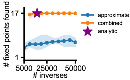
This figure compares the performance of three methods for finding fixed points in a piecewise-linear recurrent neural network: an analytic method (purple star), an approximate method (blue dots), and a combined method (orange dots). The combined method uses Proposition 1 to constrain the search space of the approximate method. The x-axis shows the number of matrix inversions computed, and the y-axis shows the number of fixed points found. The analytic method consistently finds all 17 fixed points, while the approximate method’s performance varies significantly, often finding fewer fixed points and showing more variability across runs. The combined method improves upon the approximate method but still doesn’t consistently find all fixed points.
More on tables

This table compares the performance of the proposed method (SMC) with the state-of-the-art method (GTF) on EEG data in terms of the dimensionality of the latent dynamics, the total number of trainable parameters, and two performance metrics (Dstsp and DH). The results show that the proposed method achieves lower-dimensional latent dynamics while maintaining comparable performance.
This table compares the performance of the proposed method with the state-of-the-art method (GTF) on an EEG dataset. The comparison is based on the dimensionality of the latent dynamics, the total number of trainable parameters, and two evaluation metrics: Dstsp and DH. The results show that the proposed method achieves lower dimensionality while maintaining similar performance to GTF.
Full paper#

