↗ OpenReview ↗ NeurIPS Homepage ↗ Chat
TL;DR#
Scaling hyperparameter optimization in Gaussian processes (GPs) to massive datasets is a significant challenge due to the computational cost of inverting large kernel matrices. This often involves iterative methods relying on linear system solvers, but slow convergence can hinder their effectiveness. Existing methods focus on sparse approximations, which can compromise model flexibility and accuracy.
This work presents three key improvements applicable across different linear system solvers, such as conjugate gradients and stochastic gradient descent. These are: 1) a pathwise gradient estimator, amortizing the prediction cost and reducing solver iterations; 2) warm starting to accelerate convergence by reusing previous solutions; and 3) early stopping with warm starting to manage compute budgets effectively. The authors demonstrate significant speedups (up to 72x) while maintaining predictive performance across various datasets and solvers.
Key Takeaways#
Why does it matter?#
This paper is crucial for researchers working with large-scale Gaussian processes. It offers significant speed improvements for hyperparameter optimization, a major bottleneck in GP applications. The proposed techniques are broadly applicable, impacting various fields that rely on GPs, and open avenues for further research into efficient GP inference. Addressing the scalability challenges of GPs is a major trend in machine learning, making this work highly relevant.
Visual Insights#

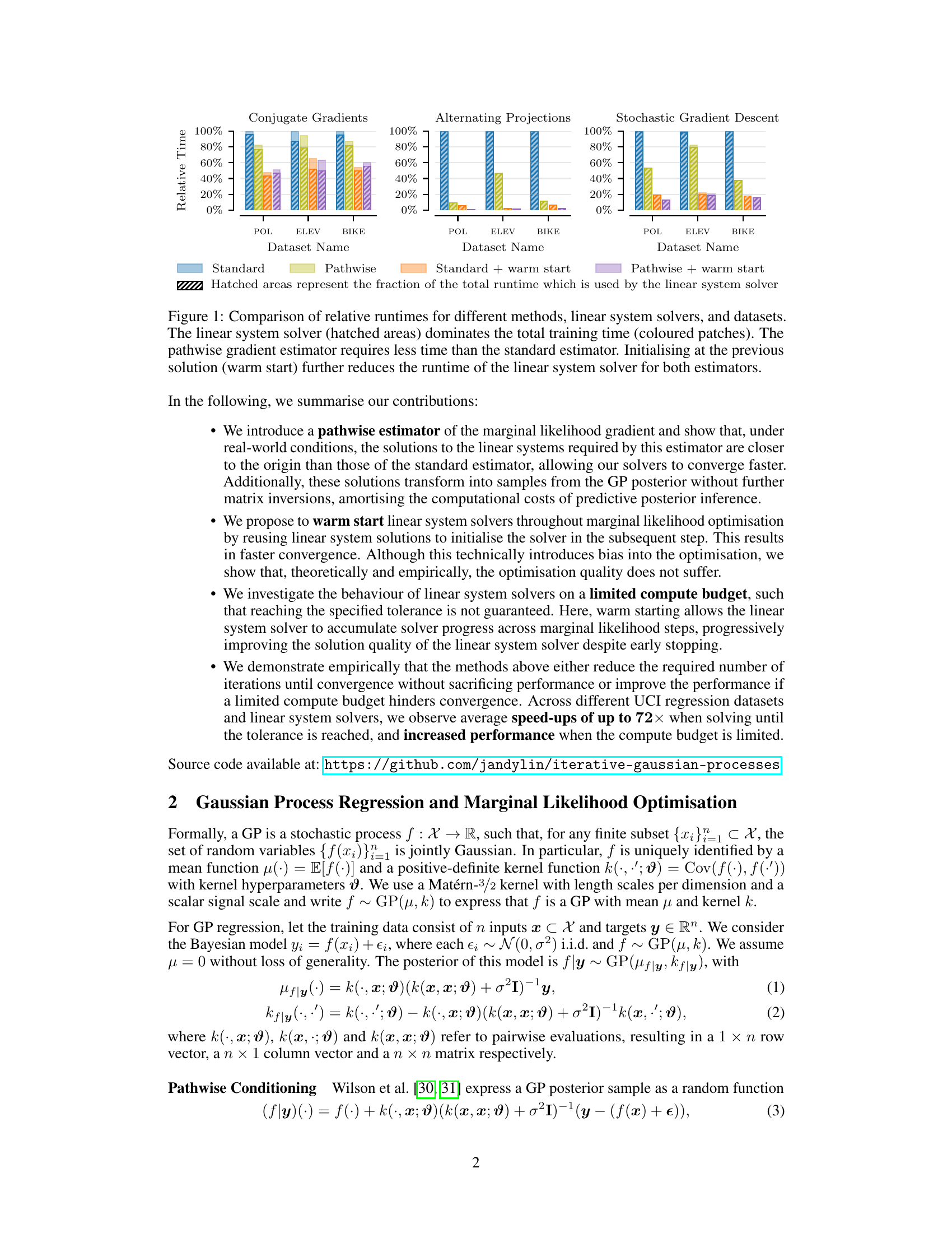
This figure compares the relative runtimes of different hyperparameter optimization methods using various linear system solvers on several datasets. The results show that the time spent on the linear system solver is the most significant portion of the overall training time. Using the pathwise gradient estimator is faster than using the standard estimator. Additionally, initializing the solver with the solution from the previous step (warm starting) further reduces the runtime.

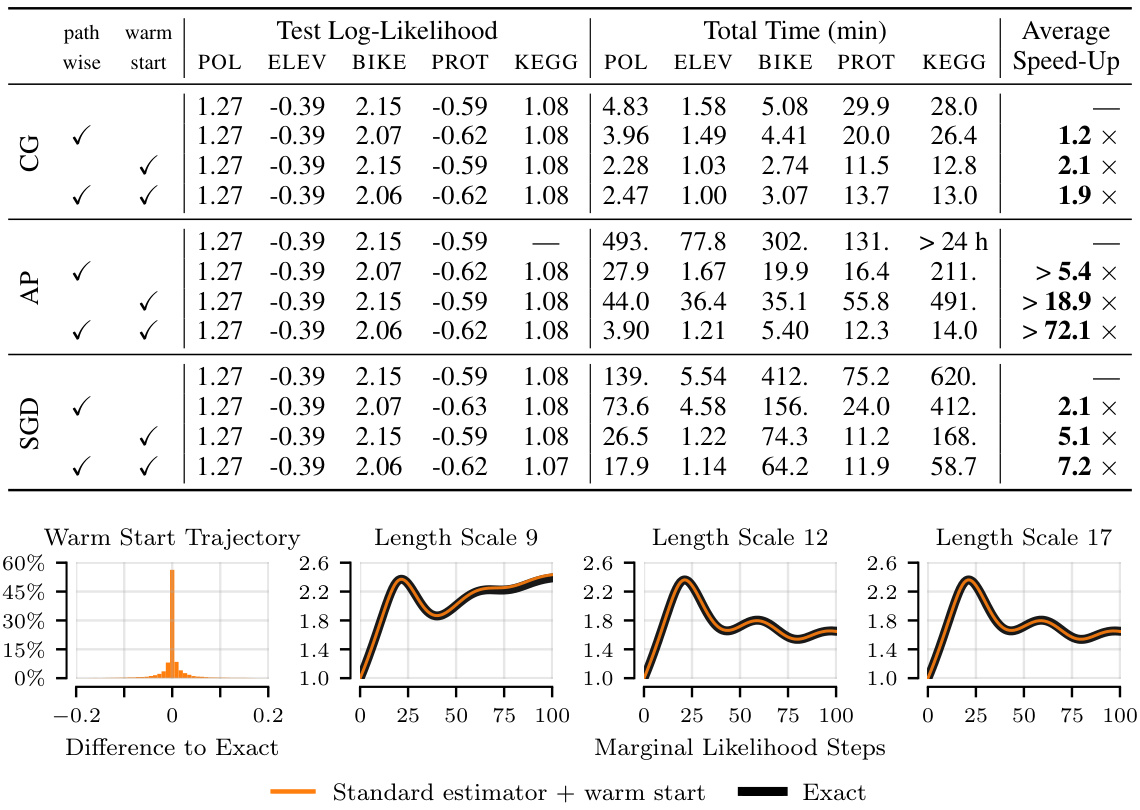
This table presents the results of applying three different linear system solvers (Conjugate Gradients, Alternating Projections, and Stochastic Gradient Descent) to the problem of hyperparameter optimization in iterative Gaussian Processes. The table shows the test log-likelihood, total training time, and speedup achieved by each solver across five different datasets, with and without two proposed optimizations (pathwise estimator and warm start). The experiment involves 100 outer-loop marginal likelihood optimization steps with a learning rate of 0.1, and only datasets with fewer than 50,000 data points are included to ensure that the solvers can reach the tolerance. The mean performance across 10 data splits is reported.
In-depth insights#
Pathwise Estimation#
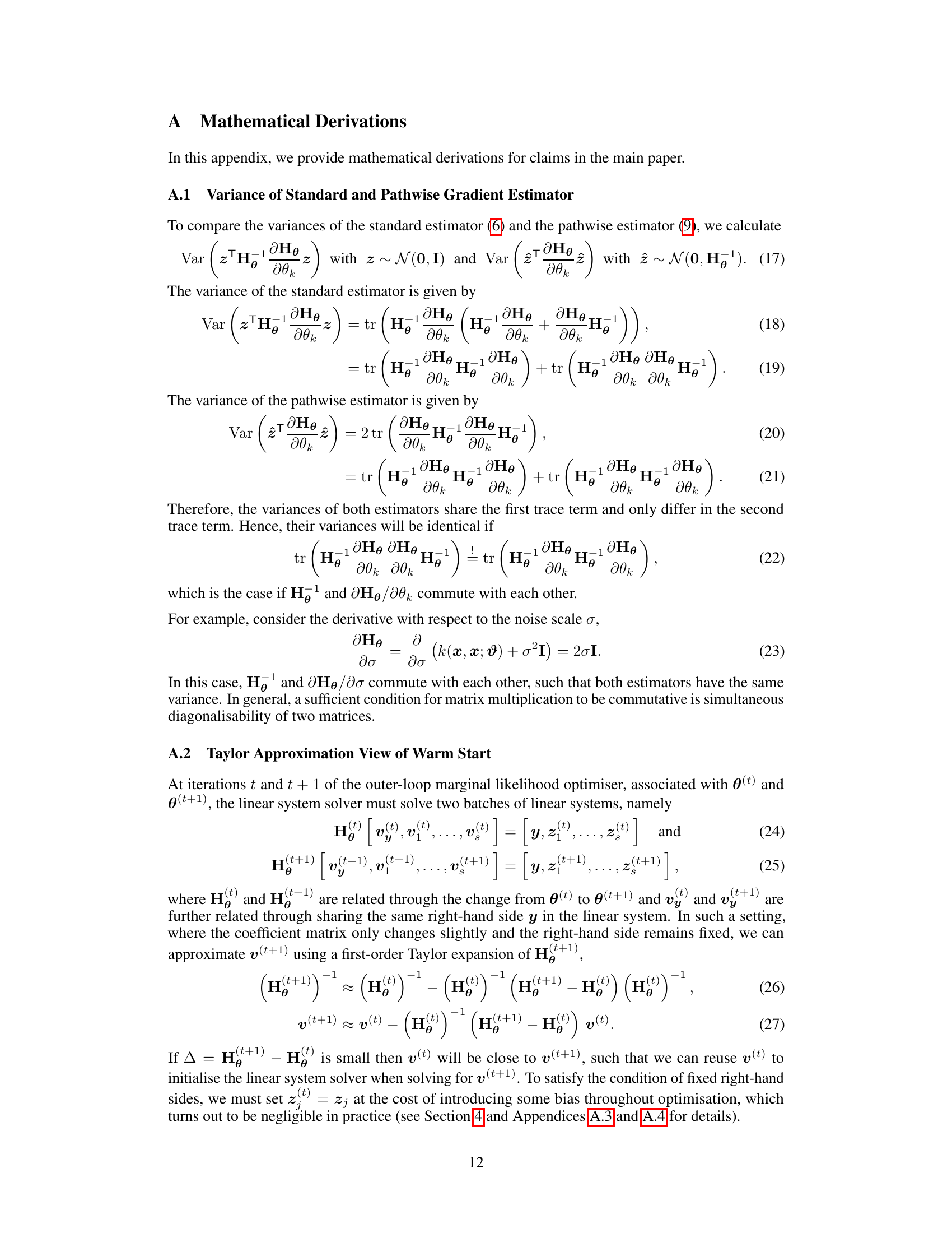
Pathwise estimation, in the context of Gaussian Processes, offers a compelling approach to enhance the efficiency of marginal likelihood optimization. By cleverly incorporating pathwise conditioning, it directly integrates the solution of linear systems into the gradient estimation process, eliminating redundant computations. This results in a substantial reduction in the number of iterations required for solver convergence and significantly decreases computational costs. The method’s effectiveness stems from its ability to generate posterior samples directly from the linear system solutions, thus amortizing the cost of predictive inference. However, careful consideration must be given to the potential introduction of bias arising from incorporating prior function samples. While theoretical and empirical results demonstrate negligible bias in practice, further investigation into its potential effects on the optimization trajectory is warranted. The method’s performance is further enhanced when combined with warm starting, but this also introduces the risk of correlated gradient estimates. Overall, the benefits of pathwise estimation, including increased efficiency, reduced computational burden and amortized inference, make it a significant advancement in iterative Gaussian Process methods.
Warm Start Solvers#
The concept of “Warm Start Solvers” in the context of iterative Gaussian processes for hyperparameter optimization is a powerful technique to accelerate convergence. By initializing the solver at the solution obtained from the previous optimization step, rather than starting from scratch (e.g., zero), warm starting leverages the inherent correlation between consecutive optimization steps. This approach significantly reduces the number of iterations required to reach a given tolerance, thus saving substantial computation time. The method’s effectiveness stems from the fact that successive optimization iterations often produce solutions close to each other. However, warm starting introduces a minor bias into the optimization procedure since the solver’s starting point is slightly shifted. Empirically, the paper shows this bias to be negligible while delivering notable speedups. The synergy between warm starting and other proposed techniques, such as early stopping and a pathwise gradient estimator, further enhances the performance gains, making it a particularly valuable contribution in dealing with large datasets where computation is a bottleneck. Careful consideration of the trade-off between speed and bias is crucial in implementing warm starting effectively.
Limited Budgets#
The section on ‘Limited Budgets’ explores a crucial real-world scenario where the computational resources for solving linear systems within iterative Gaussian Processes are constrained. The authors highlight the practical limitations of aiming for perfect solver convergence (reaching a specific tolerance) when dealing with large datasets or poor system conditioning, situations that often lead to excessively long computation times. Instead, they investigate the impact of early stopping, where solvers are terminated before reaching the target tolerance after a predetermined number of iterations. This approach introduces a trade-off between computational cost and accuracy. Their findings reveal significant performance differences across various linear solvers under these constrained conditions. Some solvers are more robust to early stopping, while others suffer significant performance degradation. Importantly, the study emphasizes that high residual norms (a measure of solver inaccuracy) don’t always correlate with poor predictive performance. This suggests that the conventional focus on minimizing the residual norm might be overly stringent in limited-budget scenarios, and prioritizing computational efficiency might sometimes be more beneficial.
Large Dataset Tests#
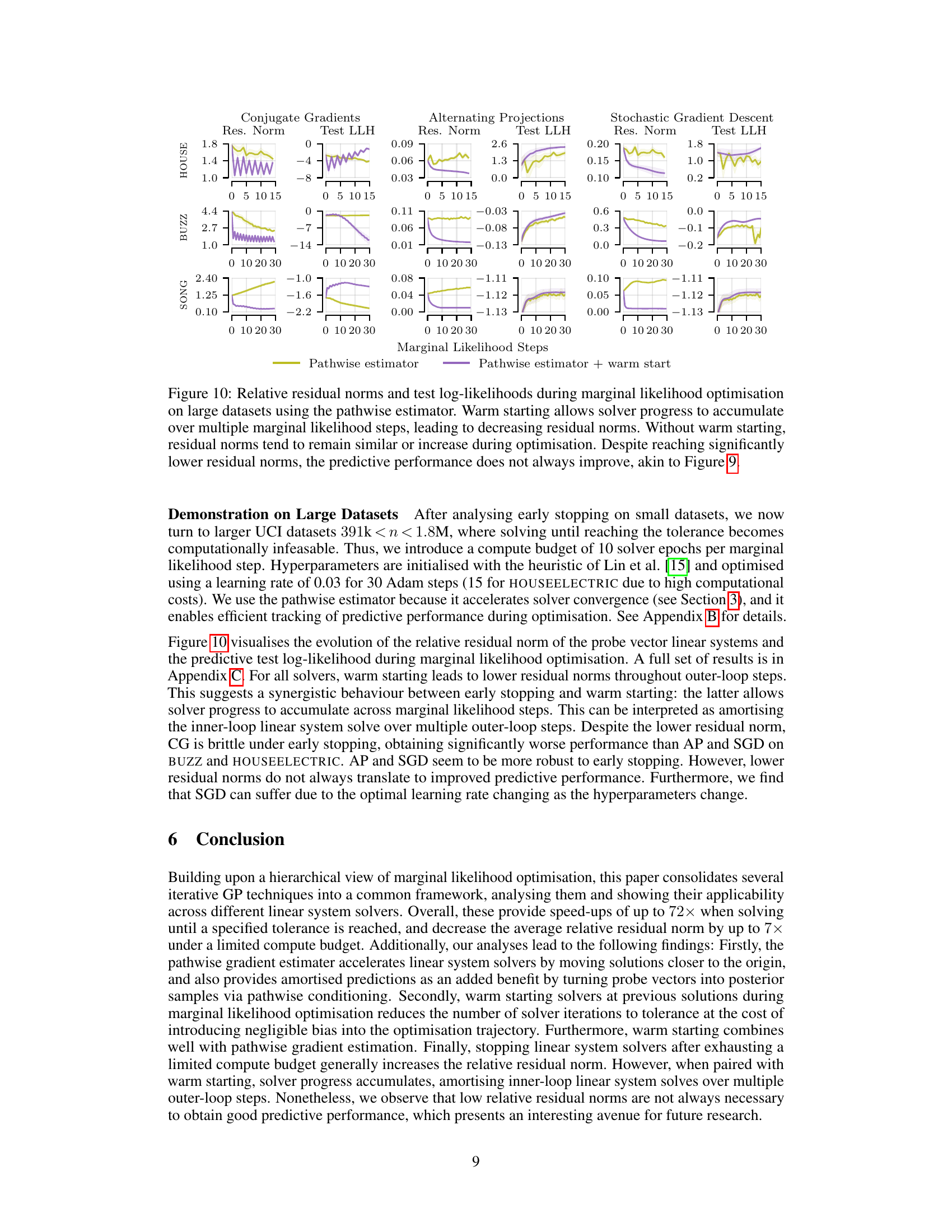
A hypothetical section titled ‘Large Dataset Tests’ in a research paper on improving linear system solvers for hyperparameter optimization in iterative Gaussian processes would explore the scalability and performance of the proposed methods on datasets significantly larger than those used in initial experiments. It would be crucial to demonstrate the effectiveness of techniques like pathwise gradient estimation, warm starting, and early stopping in reducing computational costs while maintaining predictive accuracy. The results might show speedups on datasets with millions of data points, highlighting the practical advantages of the optimized methods for real-world applications. Comparisons with existing sparse methods would also be valuable, demonstrating how the iterative approach maintains accuracy at a competitive cost. A key aspect would be demonstrating the robustness of the techniques in the presence of poor system conditioning inherent in very large datasets and comparing the performance of different solvers under compute constraints. Detailed analysis of runtime, residual norms, and predictive performance metrics across various datasets would provide strong evidence supporting the claims of the paper.
Future Work#
The paper significantly advances iterative Gaussian process methods, but several avenues for future work emerge. Extending the pathwise approach to other kernel types and GP models beyond regression is crucial to broaden its applicability. Investigating the theoretical properties of warm starting in more detail particularly regarding its effect on convergence rate and potential bias in non-convex scenarios, is important. The impact of early stopping on various solver types should be further explored with a focus on developing adaptive early-stopping criteria that balance speed and accuracy. Finally, the scaling to massive datasets beyond the current limitations should be prioritized, perhaps by combining iterative methods with more sophisticated sparse approximation techniques. Addressing these points would enhance the practicality and effectiveness of iterative GP methods for large-scale hyperparameter optimization and prediction tasks.
More visual insights#
More on figures
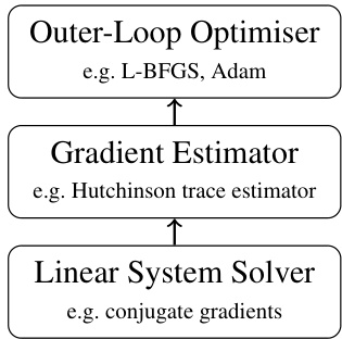
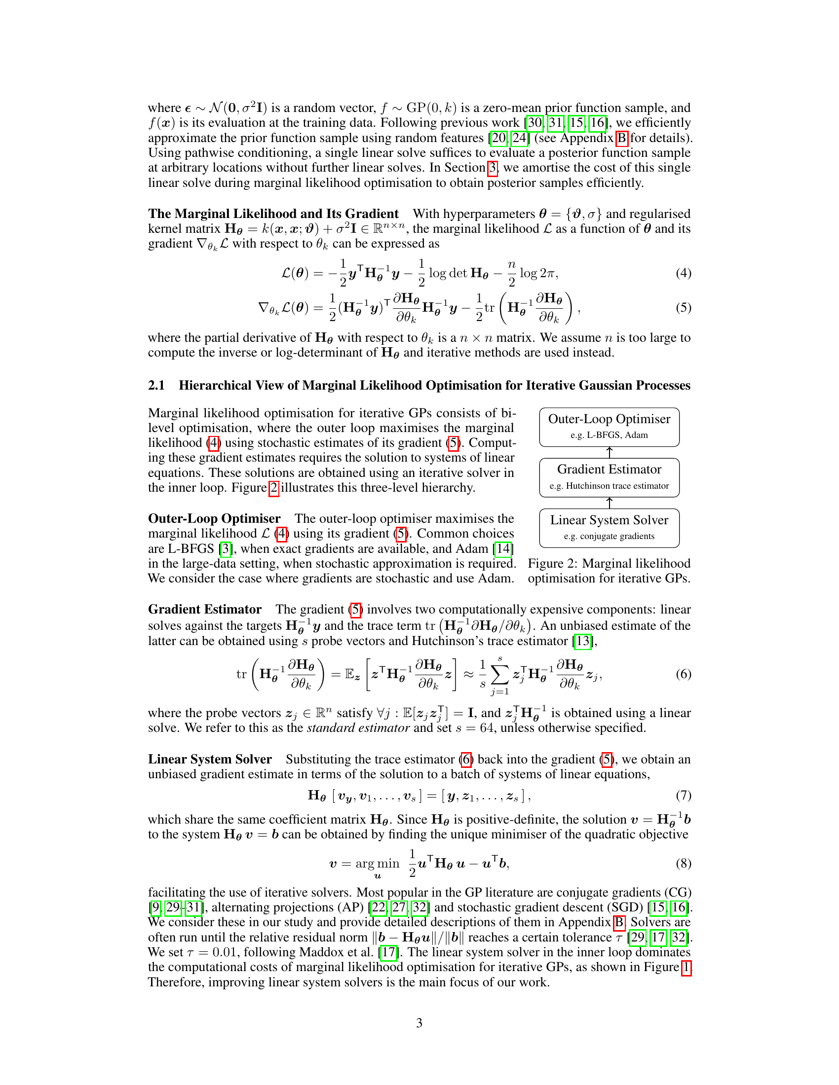
This figure illustrates the three-level hierarchical structure of marginal likelihood optimisation for iterative Gaussian processes. The outer loop uses an optimizer (like L-BFGS or Adam) to maximize the marginal likelihood. The gradient estimator (e.g., Hutchinson trace estimator) computes the gradient of the marginal likelihood, which requires solving systems of linear equations. The inner loop utilizes a linear system solver (e.g., conjugate gradients) to obtain approximate solutions to these linear systems.
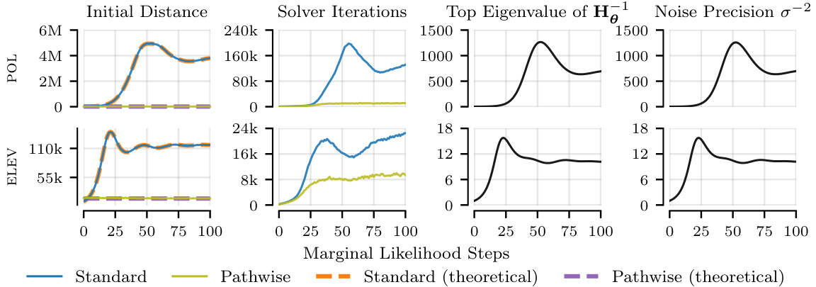
This figure compares the pathwise and standard estimators in terms of the initial distance to the solution in RKHS, the number of iterations to reach the tolerance, and the top eigenvalue of the inverse kernel matrix. The pathwise estimator demonstrates a smaller initial distance and fewer iterations, especially noticeable on the POL dataset with higher noise precision.

The figure compares the relative runtimes of different hyperparameter optimization methods using various linear system solvers across different datasets. It shows that the linear system solver is the most time-consuming part of the process. The pathwise gradient estimator significantly reduces the runtime compared to the standard estimator. Further runtime improvements are observed when using warm starting (initializing the solver with the solution from the previous step).

This figure compares the relative runtimes of different hyperparameter optimization methods using various linear system solvers (Conjugate Gradients, Alternating Projections, Stochastic Gradient Descent) on three datasets (POL, ELEV, BIKE). The hatched areas represent the proportion of total runtime spent on the linear solver itself, illustrating its dominant role. The results show that the pathwise gradient estimator significantly reduces the time compared to the standard estimator. Furthermore, warm-starting the solver (initializing it with the solution from the previous iteration) provides additional runtime improvements for both estimators.

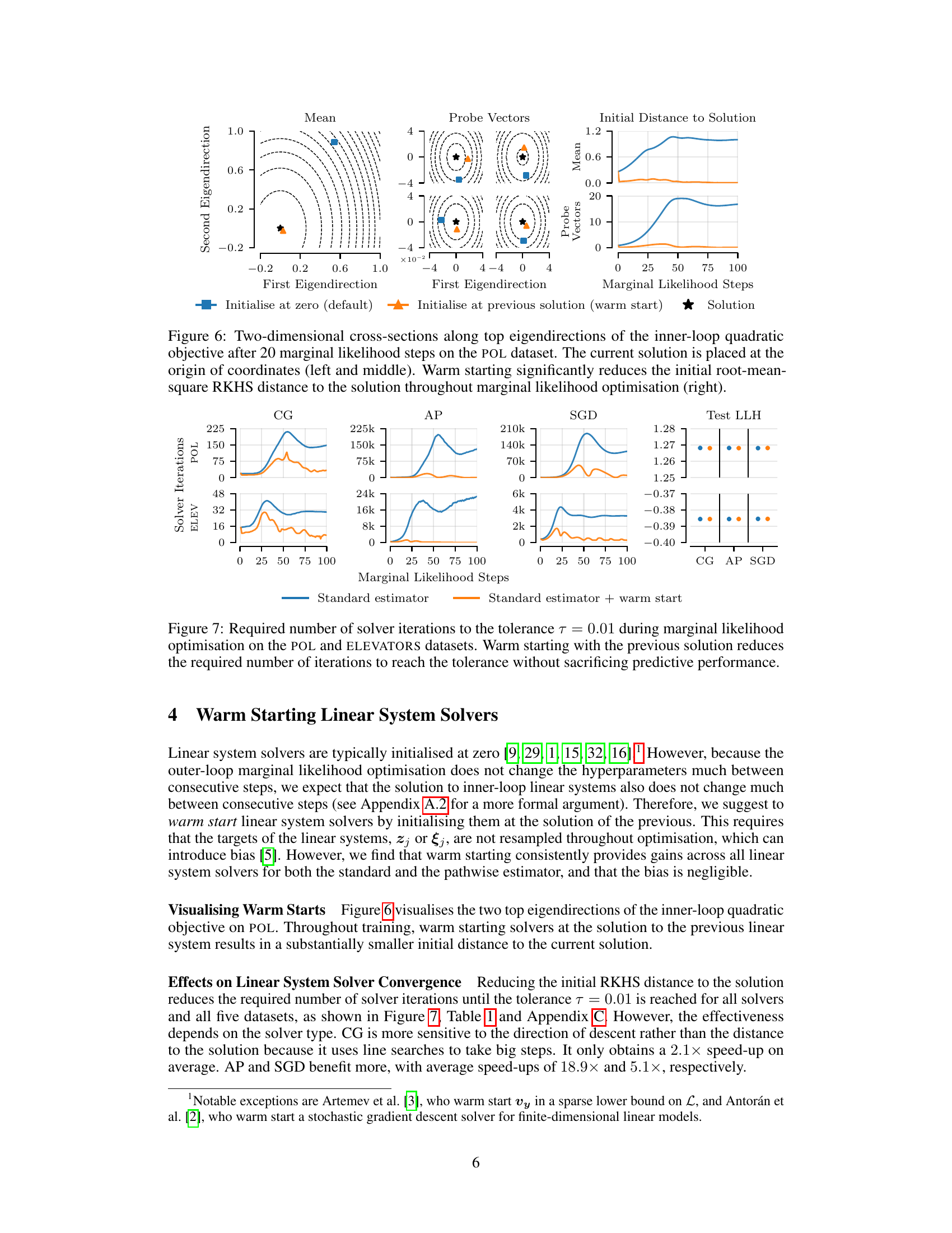
This figure visualizes the effect of warm starting on linear system solvers. It shows two-dimensional cross-sections of the quadratic objective function’s landscape for both standard initialization (at zero) and warm starting (using the previous solution) after 20 optimization steps. The left and middle panels illustrate the position of the initial point and solution for both methods. The right panel shows how warm starting reduces the initial distance to the solution over multiple optimization steps. The results demonstrate that warm starting leads to faster convergence of the solvers.

The figure compares the relative runtimes of different hyperparameter optimization methods using three different linear system solvers (Conjugate Gradients, Alternating Projections, and Stochastic Gradient Descent) on three different datasets. The results show that the pathwise gradient estimator and warm starting the linear system solver significantly reduce the runtime compared to the standard methods.
The figure compares the relative runtimes of different hyperparameter optimization methods using various linear system solvers across multiple datasets. It demonstrates that the time spent on the linear system solver is the primary contributor to the overall training time. Using a pathwise gradient estimator significantly reduces the runtime compared to the standard estimator. Furthermore, warm-starting the linear system solver (initializing it with the previous solution) provides additional speed-ups.

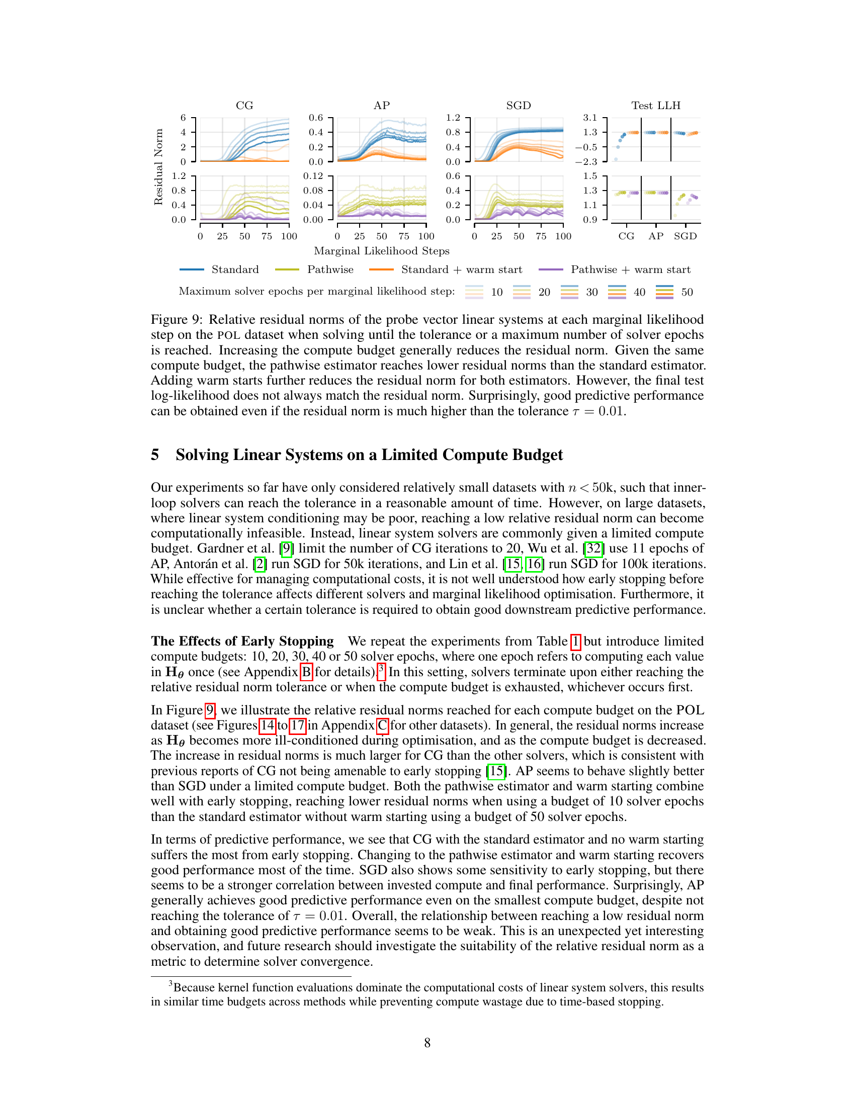
This figure shows the relative residual norms of the probe vectors for the linear systems at each marginal likelihood optimization step on the POL dataset. The results are shown for different methods (standard, pathwise, standard + warm start, pathwise + warm start) and maximum numbers of solver epochs (10, 20, 30, 40, 50). The figure demonstrates that increasing the compute budget (i.e., number of solver epochs) generally reduces the residual norm, and that the pathwise estimator and warm starting further improve the residual norm. Interestingly, good predictive performance is observed even when the residual norm is significantly higher than the tolerance (0.01).

This figure compares the relative runtimes of different hyperparameter optimization methods using various linear system solvers across different datasets. The results highlight that the linear system solver’s runtime significantly impacts the overall training time. The pathwise gradient estimator consistently outperforms the standard estimator by reducing solver runtime, and warm starting further enhances the performance by leveraging previous solutions to initialize the solver.
This figure compares the relative runtimes of different hyperparameter optimization methods using various linear system solvers across several datasets. The main takeaway is that the pathwise gradient estimator and warm starting significantly reduce the time spent on linear system solves, which is the dominant factor in the total training time.

This figure compares the relative runtimes of different hyperparameter optimization methods using various linear system solvers on three different datasets. It shows that the time spent on the linear system solver is the dominant factor in the total training time. The pathwise gradient estimator significantly reduces the runtime compared to the standard estimator, and warm-starting the solver further improves performance.

This figure compares the relative runtimes of different hyperparameter optimization methods using various linear system solvers across several datasets. The main observation is that the time spent on the linear solver is the dominant factor in the total training time. The figure shows that using the pathwise gradient estimator, along with warm starting the solver (initializing it with the solution from the previous step), significantly reduces the runtime compared to the standard method without warm starting.
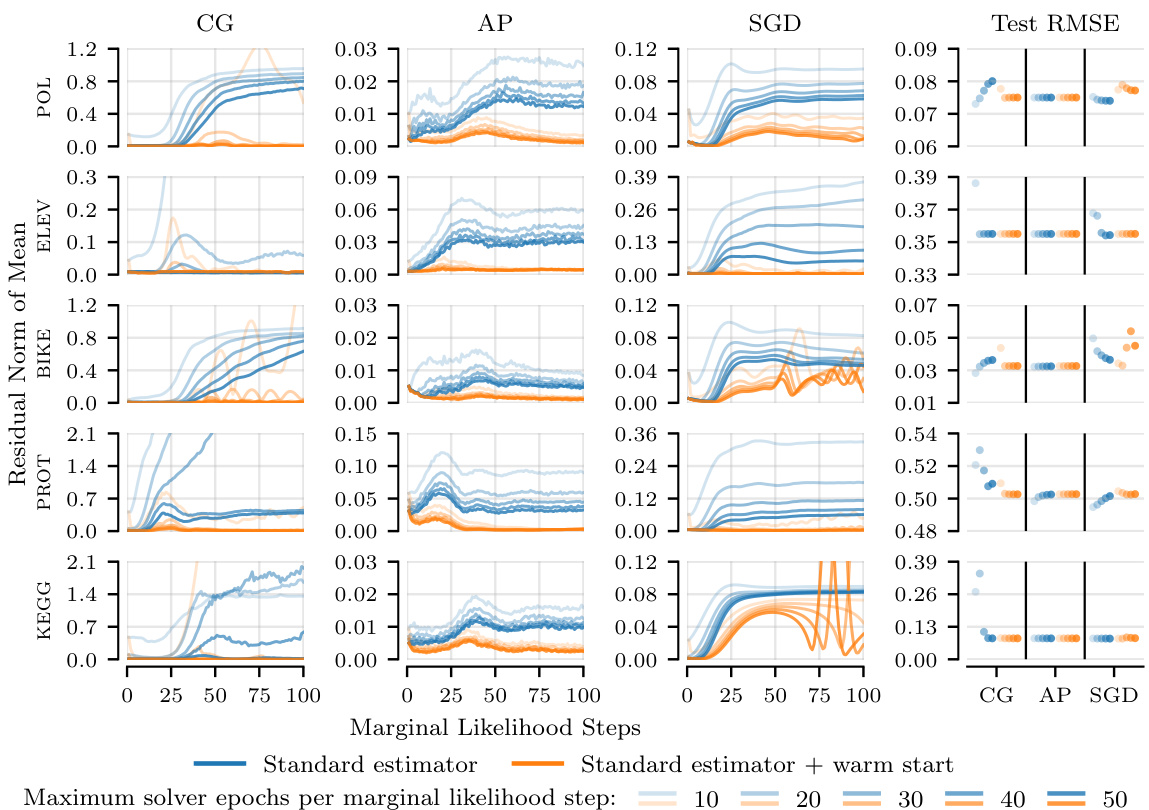
This figure compares the relative runtimes of different hyperparameter optimization methods using various linear system solvers across several datasets. The results show that the linear system solver is the dominant factor in the overall training time. The pathwise gradient estimator significantly reduces runtime compared to the standard estimator. Furthermore, warm-starting the solver with the previous solution provides additional runtime improvements for both estimators.
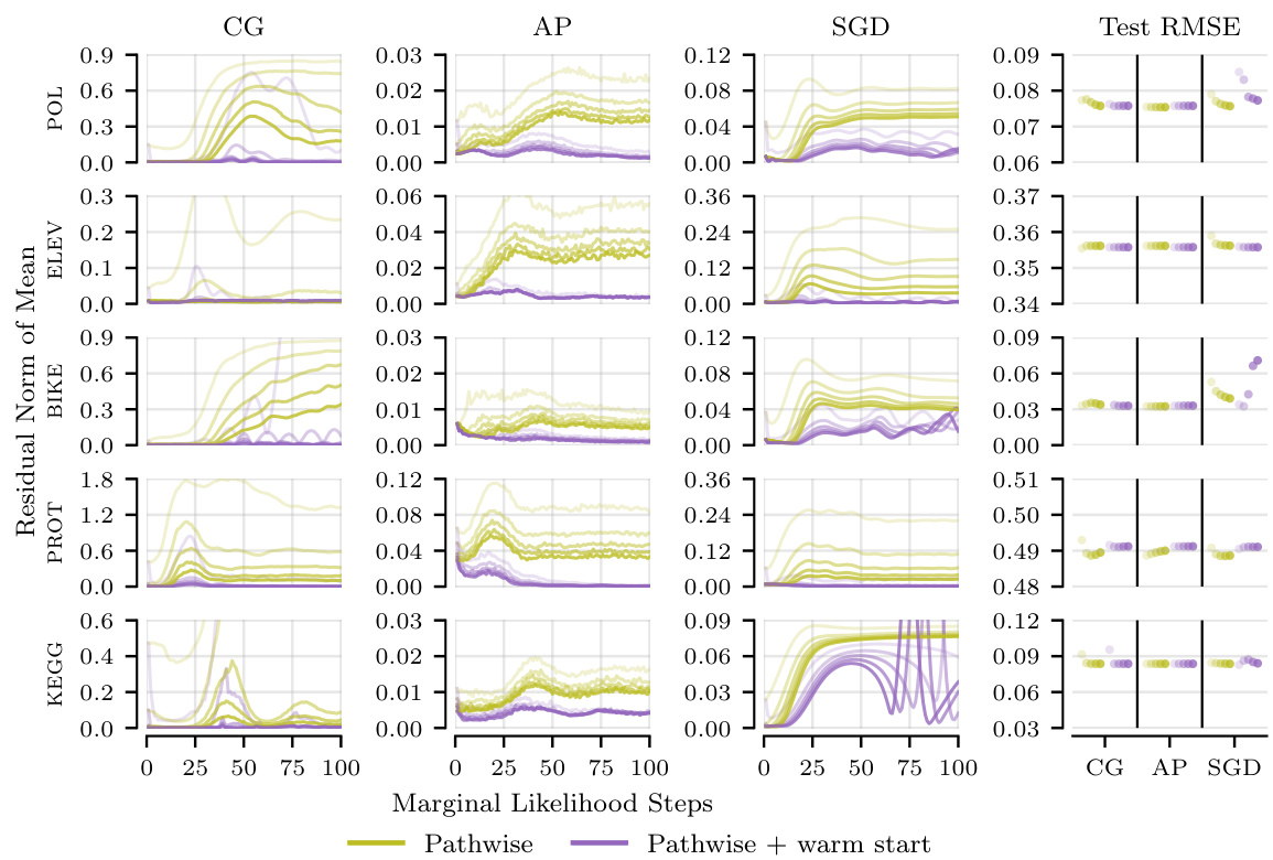
This figure compares the relative runtimes of different hyperparameter optimization methods using various linear system solvers across several datasets. It shows that the time spent on the linear system solver is the dominant factor in overall runtime. The pathwise gradient estimator offers significant speedups compared to the standard estimator. Furthermore, warm-starting the solver (using the solution from the previous step) yields additional improvements in computational efficiency.
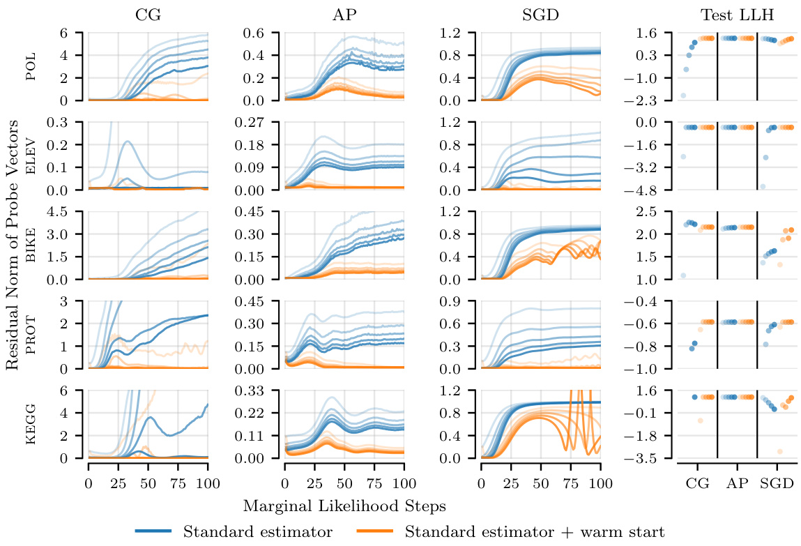
The figure compares the relative runtimes of different hyperparameter optimization methods using three different linear system solvers (Conjugate Gradients, Alternating Projections, and Stochastic Gradient Descent) across three different datasets. The main observation is that the time spent on the linear system solver dominates the overall training time. The pathwise gradient estimator significantly reduces runtime compared to the standard estimator. Further improvements are obtained by initializing the solver with the solution from the previous step (warm start).
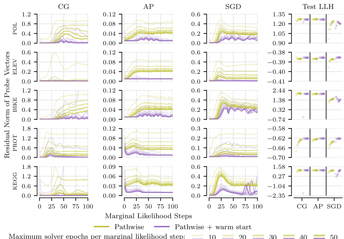
This figure shows how the residual norms of probe vectors in linear systems behave when solving until a tolerance or a maximum number of epochs is reached. The results are shown for different solvers (CG, AP, SGD) and for two gradient estimators (standard, pathwise), with and without warm starting. It shows that increasing the computation budget reduces the residual norm, and that the pathwise estimator with warm starting achieves the lowest norms. Surprisingly, good prediction performance can be achieved even when the norms are substantially larger than the target tolerance.
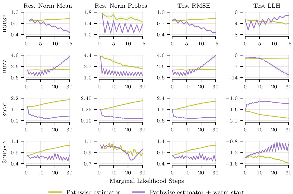
This figure shows the relative residual norms of probe vectors in linear systems for different solvers (CG, AP, SGD) at each marginal likelihood optimization step on the POL dataset. The experiment compares the standard and pathwise estimators, with and without warm starts, under varying computational budgets (maximum solver epochs). The results demonstrate that increasing the compute budget generally lowers residual norms. The pathwise estimator consistently achieves lower residual norms than the standard estimator for the same budget. Warm starting further improves performance. Interestingly, while lower residual norms are generally better, the figure also shows that good predictive performance can be maintained even with higher-than-tolerance residual norms.
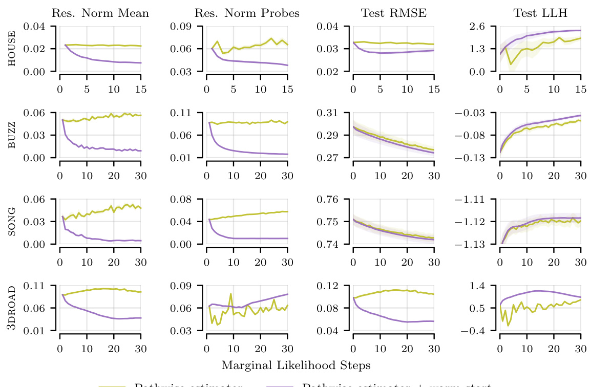
This figure compares the relative residual norms (the difference between the actual and estimated solutions) of linear systems for three different solvers (Conjugate Gradients, Alternating Projections, and Stochastic Gradient Descent) using different configurations (standard, pathwise, warm start, and pathwise + warm start) on the POL dataset. The x-axis represents the marginal likelihood steps, and the y-axis shows the relative residual norm. The figure demonstrates that increasing the computational budget (allowing more solver epochs) reduces the residual norm across all configurations. The pathwise estimator consistently achieves lower residual norms compared to the standard estimator for the same computational budget. Furthermore, incorporating warm starts further improves the residual norms, but surprisingly, this doesn’t always directly translate to higher test log-likelihood.
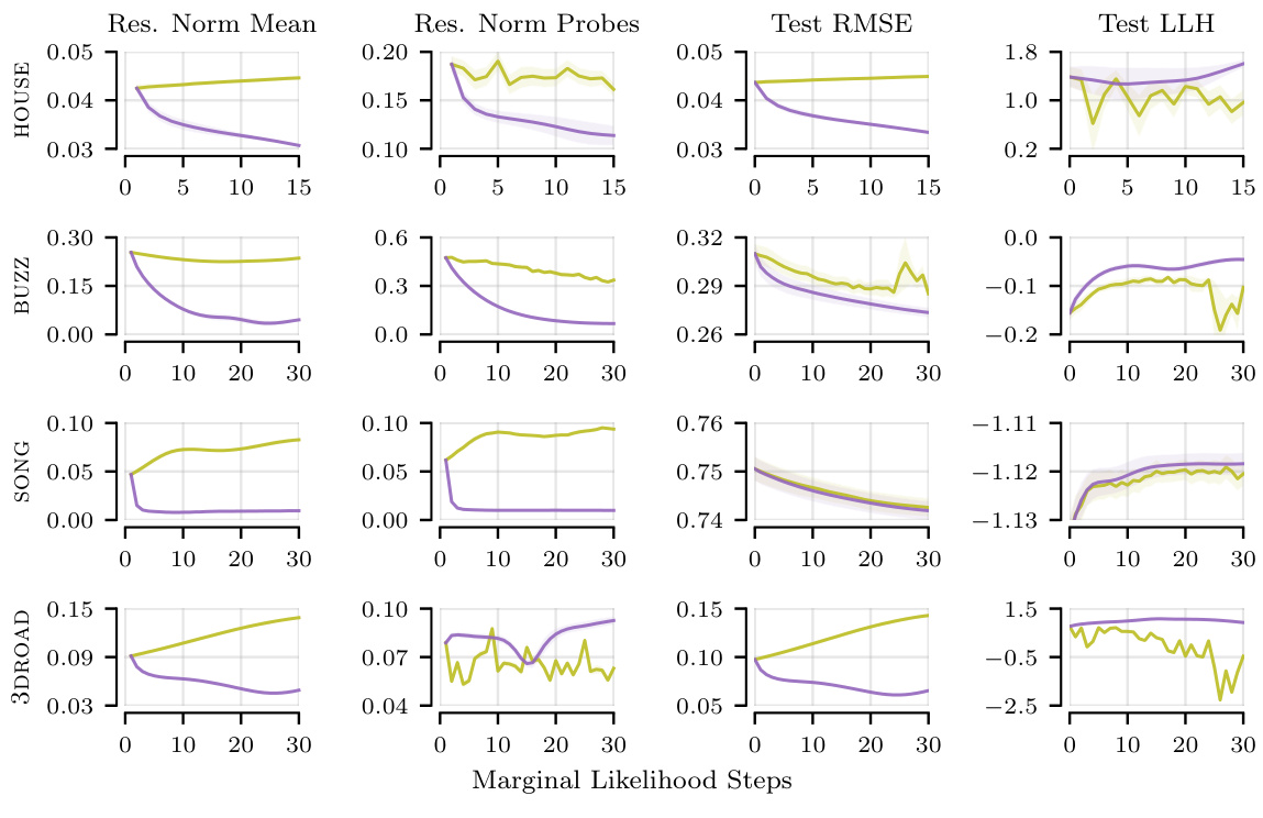
This figure compares the relative runtimes of different hyperparameter optimization methods using various linear system solvers on several datasets. The hatched areas represent the proportion of total runtime spent on the linear system solver, highlighting its dominance in overall training time. The results show that the pathwise gradient estimator is faster than the standard estimator, and that warm-starting (using the previous solution to initialize the solver) further improves speed for both estimators.
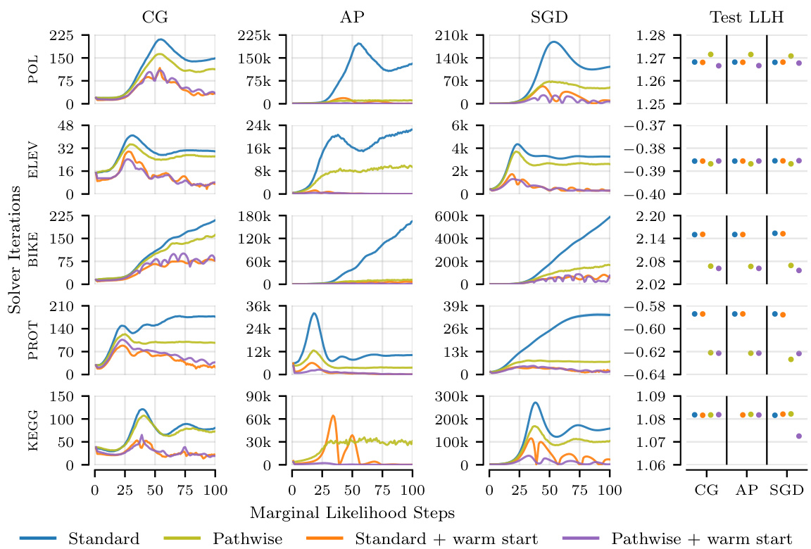
This figure compares the relative runtimes of different hyperparameter optimization methods using various linear system solvers across several datasets. The results show that the linear system solver is the most time-consuming part of the process. The pathwise gradient estimator significantly speeds up this process compared to the standard estimator, and further improvements are achieved by using warm start initialization. The improvements are substantial and evident across all three solvers (conjugate gradient, alternating projections, stochastic gradient descent).
More on tables
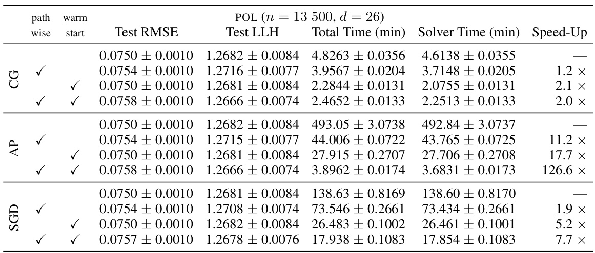
This table presents the results of three different linear system solvers (Conjugate Gradients, Alternating Projections, and Stochastic Gradient Descent) on five datasets after 100 iterations of marginal likelihood optimization. The table shows the test log-likelihood, total training time, solver time, and speed-up achieved by each solver, comparing standard and enhanced methods (pathwise and warm start). The small dataset size (n<50k) allows solving to convergence and the mean over 10 data splits is reported.

This table presents the results of three different linear system solvers (Conjugate Gradients, Alternating Projections, and Stochastic Gradient Descent) on five datasets after 100 iterations of marginal likelihood optimization. The table shows test log-likelihood, total training time, solver time, and speed-up compared to a baseline method. The datasets used all have fewer than 50,000 data points, allowing the solvers to reach a specified tolerance. Results are averaged over 10 different random data splits.

This table presents the results of the experiments conducted on five datasets with fewer than 50,000 data points. The experiments involved using three different linear system solvers (Conjugate Gradients, Alternating Projections, and Stochastic Gradient Descent) for 100 iterations of outer-loop marginal likelihood optimization with a learning rate of 0.1. The table shows the test log-likelihood, total training time, and the average speedup achieved by each solver.

This table presents the results of three different linear system solvers (Conjugate Gradients, Alternating Projections, and Stochastic Gradient Descent) on five datasets. The solvers were run for 100 iterations of marginal likelihood optimization, with a learning rate of 0.1. The table shows the test log-likelihood, total training time, solver time, and the speedup achieved by each method, averaged over 10 separate runs for each dataset. The table highlights the impact of different techniques like the pathwise estimator and warm starting on improving solver performance.
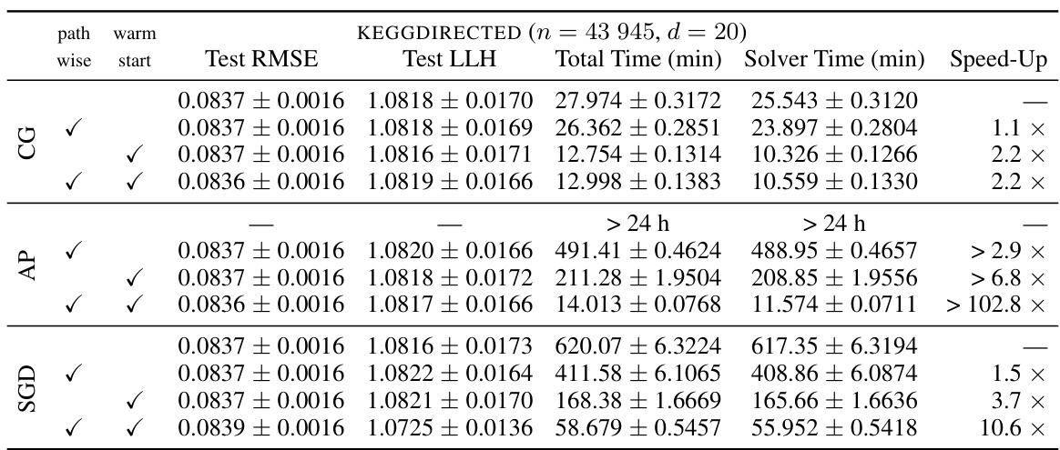
This table presents the results of three linear system solvers (Conjugate Gradients, Alternating Projections, and Stochastic Gradient Descent) on five datasets after 100 iterations of marginal likelihood optimization. It shows the test log-likelihood, total training time, solver time, and speedup achieved by each solver for various combinations of pathwise estimator usage and warm starting. The data used has less than 50,000 data points, allowing the solvers to reach convergence.

This table presents the results of experiments comparing three linear system solvers (Conjugate Gradients, Alternating Projections, and Stochastic Gradient Descent) on five datasets. The experiment involved running 100 outer-loop marginal likelihood optimization steps with a learning rate of 0.1. The table shows the mean test log-likelihood, total training time, and average speed-up achieved by each solver across the five datasets and two configurations (with and without warm start). The small dataset size allowed the solvers to reach the tolerance.

This table presents the results of applying three different linear system solvers (Conjugate Gradients, Alternating Projections, and Stochastic Gradient Descent) to the problem of hyperparameter optimization in iterative Gaussian processes. The experiment involved 100 steps of marginal likelihood optimization with a learning rate of 0.1. Five datasets with less than 50,000 data points were used, allowing the solvers to reach the tolerance. The table shows the mean test log-likelihood, total training time, solver time, and speed-up achieved for each solver across all datasets and data splits.

This table presents the results of three different linear system solvers (Conjugate Gradients, Alternating Projections, and Stochastic Gradient Descent) applied to five datasets after 100 iterations of the marginal likelihood optimization. The table shows test log-likelihood, total training time, solver time, and speedup compared to the standard approach. The small dataset size (n < 50k) ensures that solutions converge to the specified tolerance.

This table presents a comparison of the performance of three different linear system solvers (Conjugate Gradients, Alternating Projections, and Stochastic Gradient Descent) across five datasets. The solvers are used within an iterative Gaussian Process framework for hyperparameter optimization. The table shows test log-likelihood, total training time, solver time, and the speedup achieved by different techniques (pathwise estimation and warm start) relative to a standard approach. The results are averaged over 10 different random data splits for each dataset. The focus is on demonstrating improvements in efficiency while maintaining predictive performance.
Full paper#
