TL;DR#
Probabilistic forecasting of multivariate time series is often hindered by the simplifying assumption of temporally independent errors. Real-world data, however, frequently exhibits autocorrelation and cross-lag correlation due to omitted factors. Ignoring this correlation leads to inaccurate uncertainty quantification and suboptimal predictive performance. Existing deep learning models, while efficient in handling contemporaneous covariance, often fail to address this temporal dependence effectively.
This work presents a novel method to address the limitations of existing probabilistic forecasting models by explicitly modeling the covariance structure of errors over multiple steps. It employs a low-rank plus diagonal parameterization for contemporaneous covariance and independent latent processes to capture cross-covariance. This efficient parameterization enables scalable inference. The learned covariance matrix then calibrates predictions using observed residuals. The proposed method is evaluated using RNNs and Transformers, demonstrating significant improvements in predictive accuracy and uncertainty quantification, especially in multivariate settings. This method is demonstrated to be effective without adding significant model complexity.
Key Takeaways#
Why does it matter?#
This paper is crucial for researchers in probabilistic time series forecasting as it introduces a novel, efficient method for handling correlated errors in multivariate models—a common issue in real-world data that significantly impacts prediction accuracy and uncertainty quantification. The proposed approach improves prediction quality and uncertainty estimation without increasing model complexity, making it practical for large-scale applications. This opens up avenues for improved forecasting in various domains, such as finance and weather prediction.
Visual Insights#

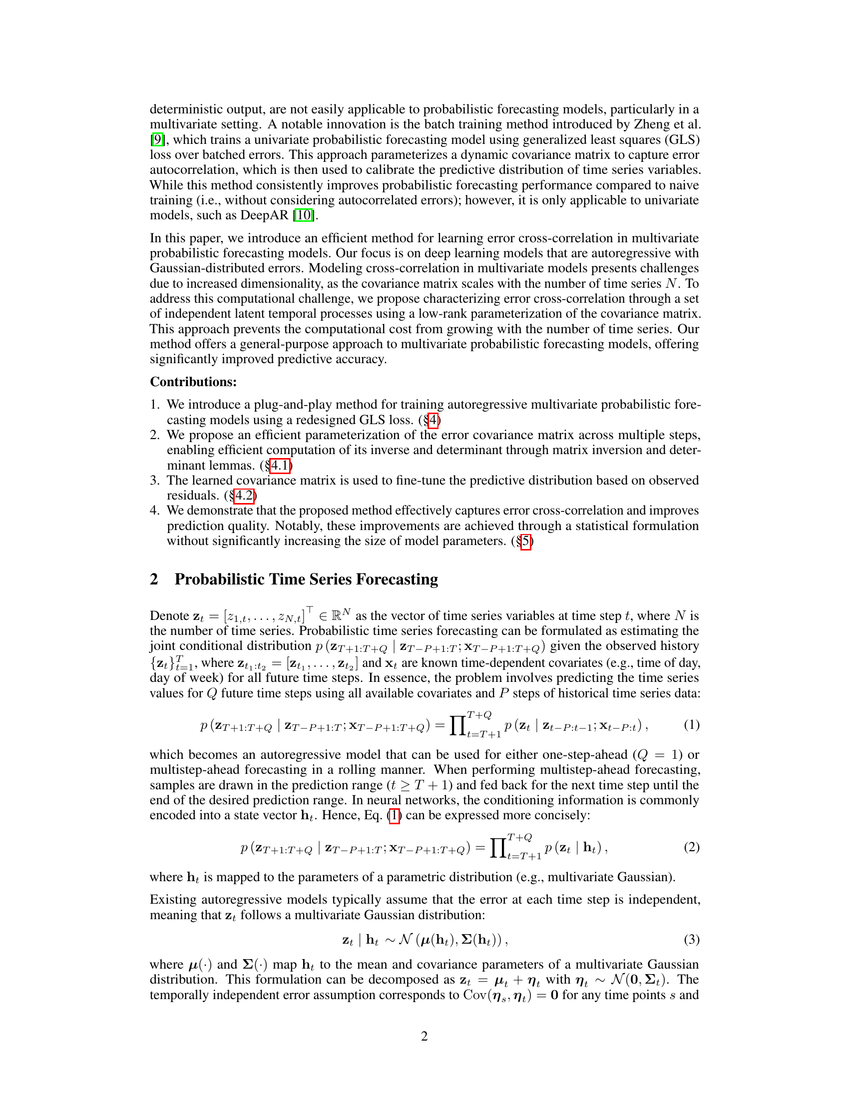
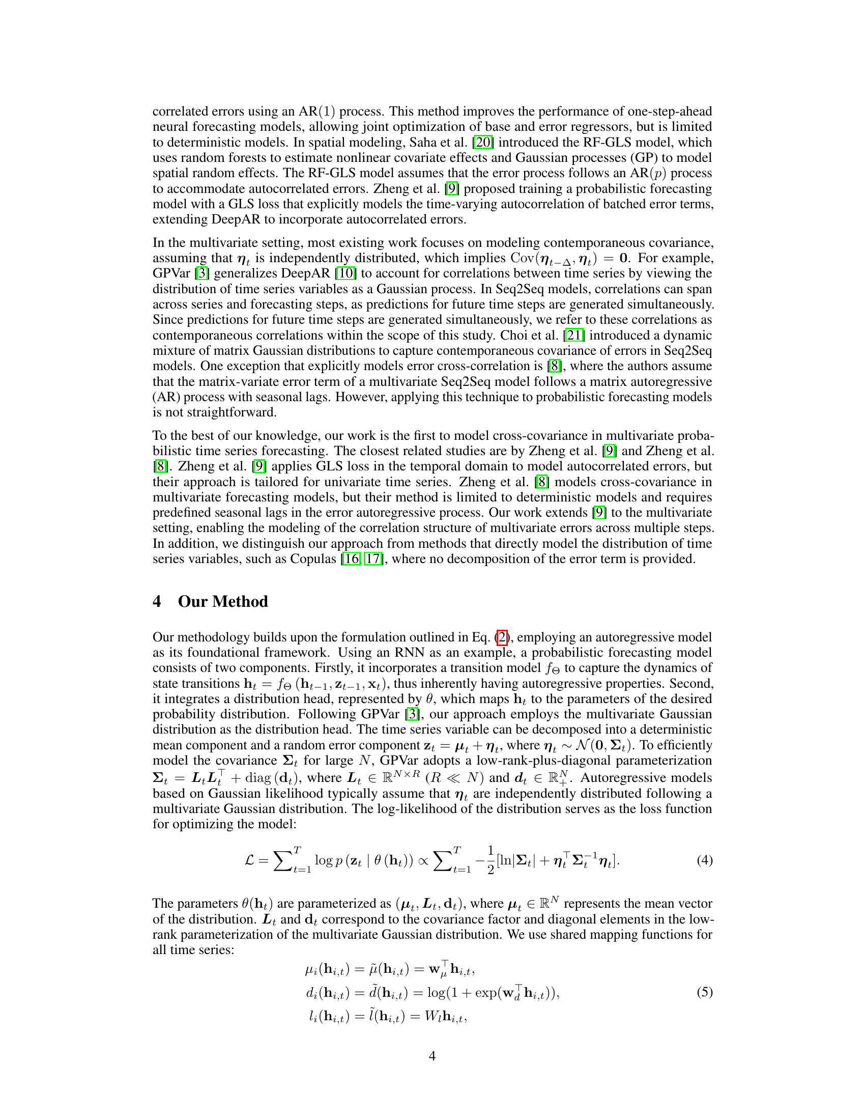
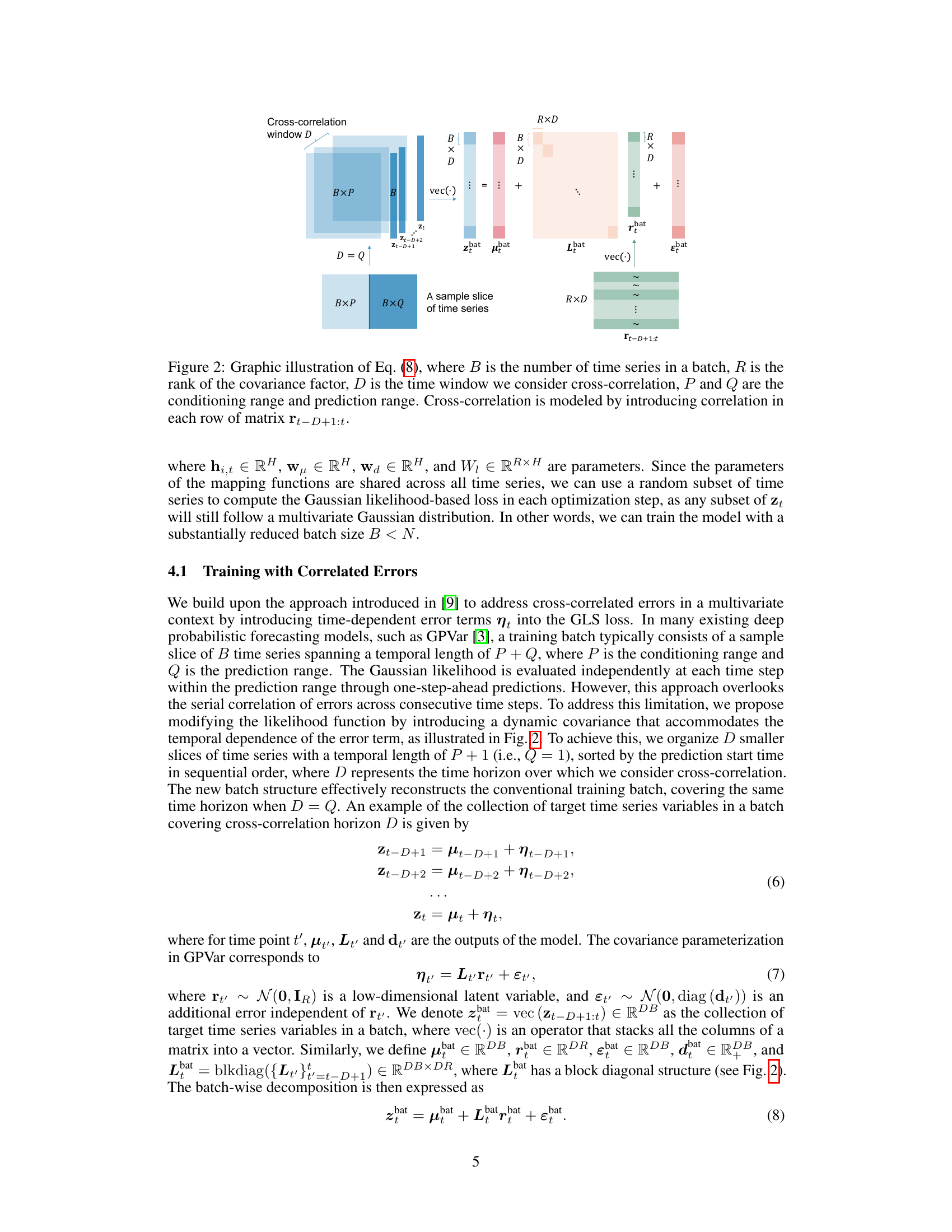
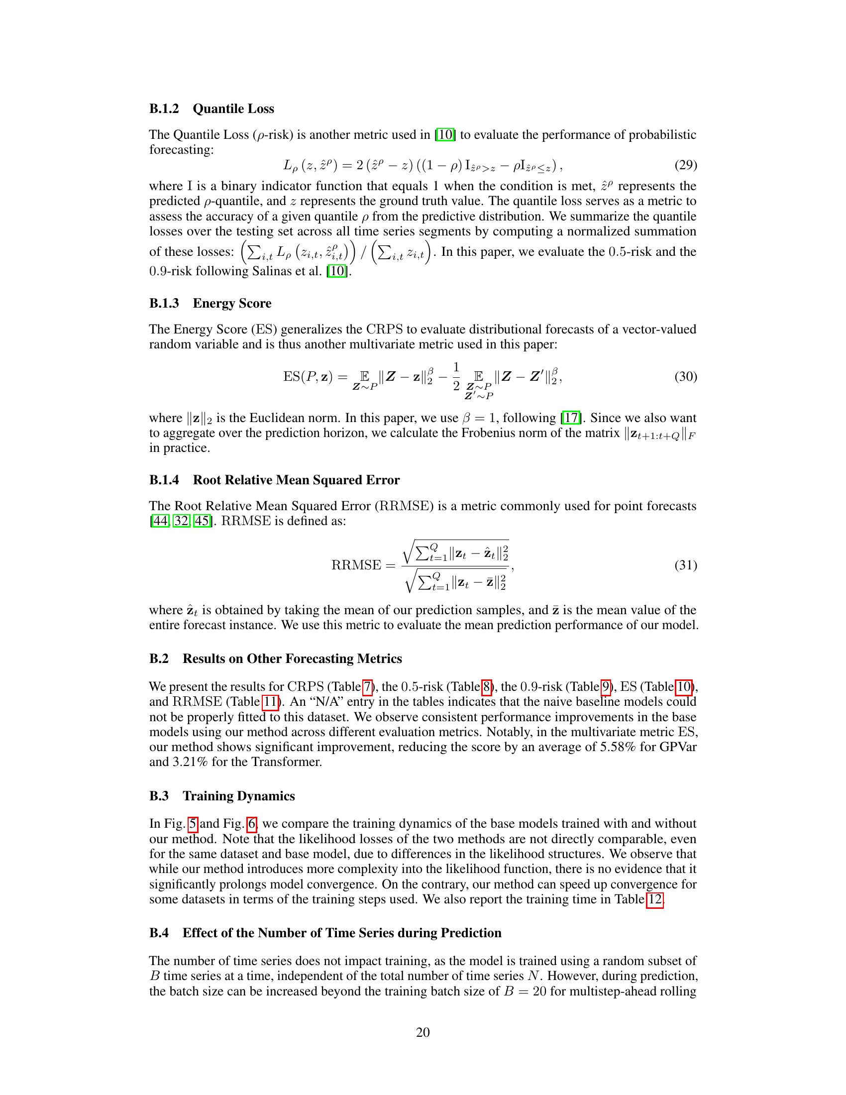
🔼 This figure shows the contemporaneous and cross-covariance matrices of prediction residuals from a multivariate time series model. The contemporaneous covariance matrix, Cov(nt, nt), displays the correlation between different time series at the same time step. The cross-covariance matrices, Cov(nt−∆, ηt) for ∆=1,2,3, show the correlation between time series at different time steps (lags). The data is from the m4_hourly dataset, and covariances are clipped for better visualization.
read the caption
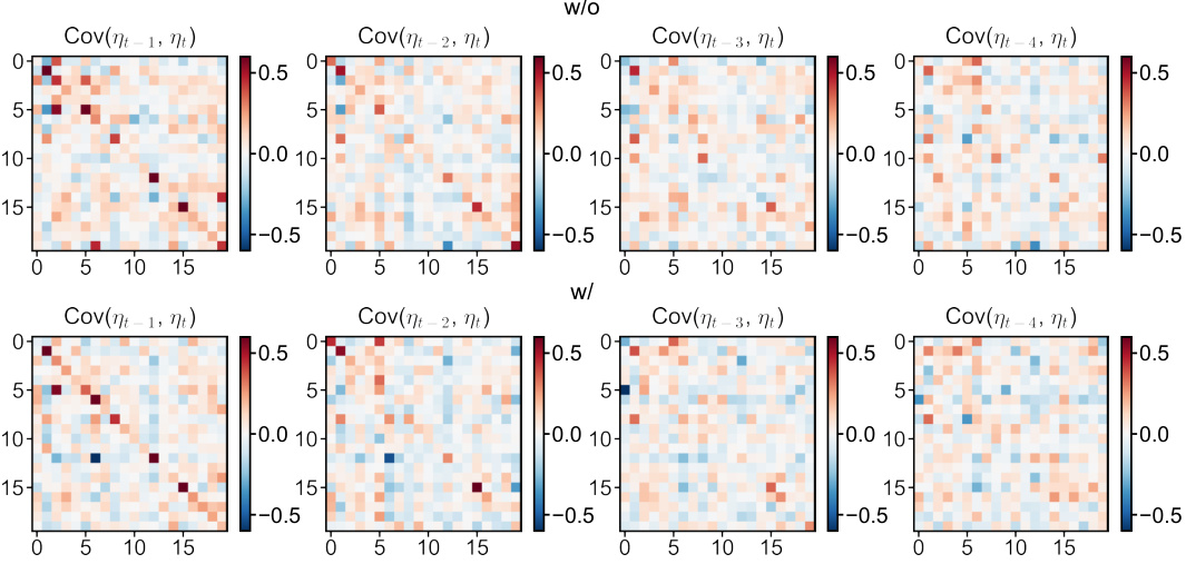
Figure 1: Contemporaneous covariance matrix Cov(nt, nt) and cross-covariance matrix Cov(nt−∆, ηt), ∆ = 1,2,3, calculated based on the one-step-ahead prediction residuals of GP-Var on a batch of time series from the m4_hourly dataset. For visualization clarity, covariance are clipped to the range [0, 0.6].

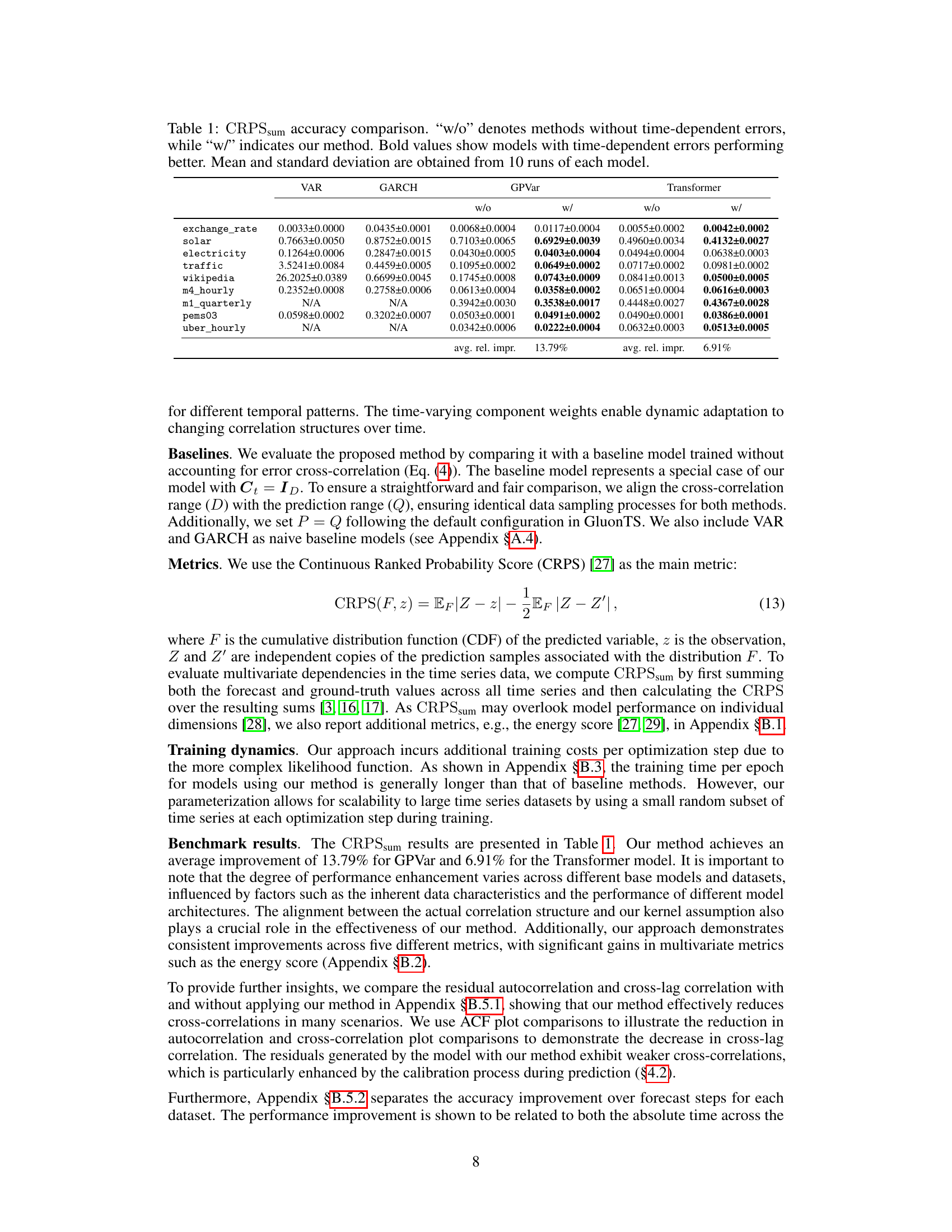
🔼 This table presents a comparison of the Continuous Ranked Probability Score (CRPS) sum across various time series datasets. Two model types are compared: those without and those with the proposed method for handling time-dependent errors. The ‘w/o’ column represents results from models without considering temporal error dependencies, while the ‘w/’ column shows results with the proposed method incorporated. Bold values highlight cases where the model incorporating time-dependent error handling outperformed its counterpart. Results are averaged over ten runs for each model.
read the caption
Table 1: CRPSsum accuracy comparison. 'w/o' denotes methods without time-dependent errors, while 'w/' indicates our method. Bold values show models with time-dependent errors performing better. Mean and standard deviation are obtained from 10 runs of each model.
In-depth insights#
Correlated Error Modeling#
The concept of correlated error modeling in time series forecasting is crucial because the assumption of independent errors often doesn’t hold in real-world scenarios. Ignoring temporal dependencies in errors leads to inaccurate uncertainty quantification and suboptimal predictive performance. The research delves into the issue of how to effectively capture both contemporaneous and cross-lag correlations across multiple time series. The challenge lies in the high dimensionality of covariance matrices involved, especially with many time series. To address this, low-rank approximations are typically used for efficient parameterization and inference. Methods for learning these covariance structures, whether employing Gaussian processes, dynamic correlation matrices, or autoregressive processes on residuals, need to balance accuracy with computational efficiency. Furthermore, the study often focuses on the problem of how best to integrate error correlation models with existing deep learning architectures. There is often a trade-off between flexibility in capturing complex correlation patterns and ease of implementation and training. The effectiveness of these methods is frequently evaluated on standard benchmarking datasets, comparing predictive accuracy with and without the consideration of correlated errors. A major theme across research is developing plug-and-play methods that can easily be incorporated into existing probabilistic models, allowing the use of improved uncertainty quantification without substantial increases in computational complexity.
Multivariate Forecasting#
Multivariate forecasting presents a significant challenge due to the complex interdependencies between multiple time series. Accurate modeling of these relationships is crucial for reliable predictions and uncertainty quantification. Traditional univariate methods fail to capture these intricate dynamics. Deep learning offers powerful tools to tackle the high dimensionality and non-linear patterns often inherent in multivariate data. However, the assumptions made, such as temporal independence of errors, often limit accuracy. Addressing error autocorrelation and cross-correlation is key to improving predictive accuracy and uncertainty estimation. Recent advancements in this field employ techniques like low-rank parameterizations and latent temporal processes to make inference computationally efficient. The choice of appropriate model architecture (RNNs, Transformers, etc.) also significantly influences performance. Furthermore, the effectiveness of multivariate forecasting depends heavily on the data’s specific characteristics, necessitating careful consideration of dataset properties and model selection. Future research directions could explore more sophisticated covariance modeling techniques and robust methods for handling non-Gaussian error distributions.
Efficient GLS Loss#
An efficient GLS loss function is crucial for probabilistic time series forecasting, particularly in multivariate settings. A naive approach would suffer from computational challenges due to the high dimensionality of the covariance matrix involved. The key to efficiency lies in clever parameterizations that reduce the computational burden without sacrificing accuracy. This might involve low-rank approximations of the covariance matrix, exploiting its structure (e.g., sparsity, Toeplitz structure), or employing efficient matrix inversion techniques (e.g., using the Sherman-Morrison-Woodbury formula). Furthermore, an efficient GLS loss would likely incorporate techniques to handle temporal dependence of errors, improving the accuracy of uncertainty quantification. This might involve modeling error autocorrelation or cross-correlation through latent variables, allowing for scalable inference and avoiding the need for inverting potentially very large covariance matrices. In summary, designing an efficient GLS loss is a multifaceted optimization problem requiring careful consideration of the computational cost and the representational power required for accurate probabilistic forecasting in a multivariate time-series context.
RNN & Transformer#
Recurrent Neural Networks (RNNs) and Transformers are prominent deep learning architectures employed for sequence modeling tasks. RNNs, particularly LSTMs and GRUs, excel at capturing temporal dependencies due to their recurrent nature. However, their sequential processing can be computationally expensive and struggle with long-range dependencies. Transformers, on the other hand, leverage the attention mechanism to process sequences in parallel, allowing for more efficient handling of long sequences and capturing global relationships. This architectural difference makes them suitable for various time series forecasting tasks. In the context of probabilistic time series forecasting, both architectures are capable of modeling the probability distribution of future values. The choice between RNNs and Transformers often depends on factors like sequence length, computational resources, and the desired level of accuracy. While RNNs offer a simpler model structure, the parallel processing capabilities of Transformers often lead to better performance on long time series. The study likely focuses on how each architecture is adapted for incorporating temporally correlated errors, leveraging either the inherent temporal modeling of RNNs or the flexibility of the Transformer’s attention mechanism. Integrating a method to incorporate error correlation into both architectures allows a comparison of their relative strengths and weaknesses in handling this challenging aspect of time series prediction.
Future Research#
The paper’s conclusion suggests several avenues for future research. Extending the model to handle non-Gaussian error distributions is crucial for improving robustness and accuracy in real-world scenarios. This could involve transforming data to achieve normality or exploring alternative distributions. Exploring more flexible covariance structures beyond the current approach is also important. The current Kronecker structure limits the model’s ability to capture complex correlation patterns. Alternatives like fully learnable Toeplitz matrices or more sophisticated coregionalization models could offer greater flexibility. Investigating the impact of different kernel functions within the dynamic covariance matrix is another area requiring further study. This could reveal optimal combinations for various time series characteristics. Finally, a comprehensive analysis of the model’s scalability and performance with respect to dataset size and prediction horizon is warranted. Future work should investigate strategies for efficiently handling very large datasets and long-term forecasts.
More visual insights#
More on figures

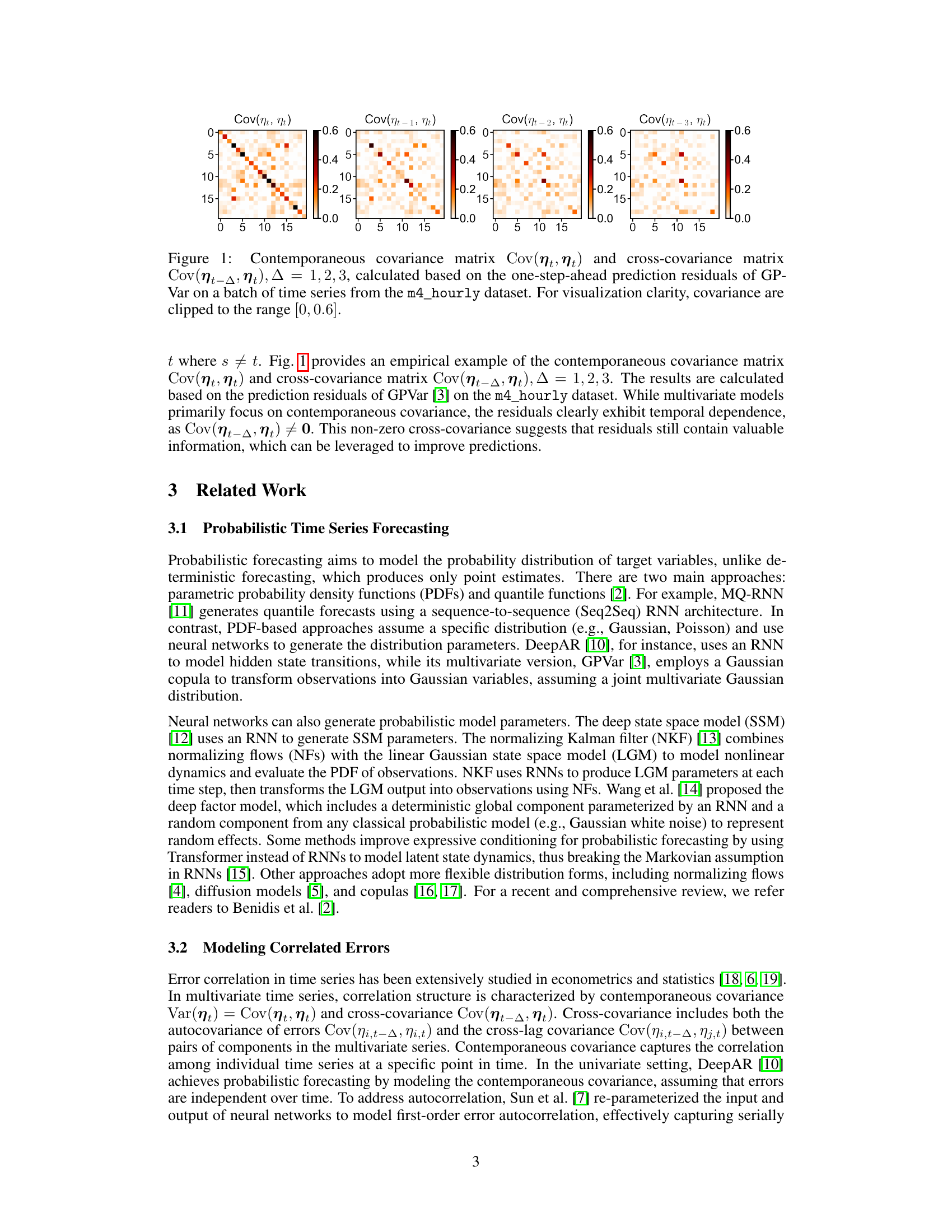
🔼 This figure illustrates how the proposed method models cross-correlation in multivariate time series. The input data is organized into a batch of time series with a specific temporal structure that spans a window of size D, encompassing both conditioning (P) and prediction (Q) ranges. The figure shows how the input data (z_bat) is decomposed into the mean (μ_bat), the low-rank covariance factor (L_bat), and a latent variable (r_bat) which models cross-covariance between different time steps and the diagonal matrix ε_bat. The key innovation shown is the use of matrix r_bat to introduce correlations across different time steps within the batch, allowing the model to learn cross-correlations.
read the caption
Figure 2: Graphic illustration of Eq. (8), where B is the number of time series in a batch, R is the rank of the covariance factor, D is the time window we consider cross-correlation, P and Q are the conditioning range and prediction range. Cross-correlation is modeled by introducing correlation in each row of matrix rt−D+1:t.

🔼 This figure illustrates how the proposed method models cross-correlation in multivariate time series. It shows a batch of time series data organized into smaller slices to capture the temporal dependencies of errors (cross-correlation). The figure highlights the components of Equation (8), showing how the cross-correlation is introduced into the latent variable vector r through a dynamic correlation matrix C. Specifically, the figure demonstrates how the cross-correlation is modeled by introducing correlation within each row of the matrix rt-D+1:t. This matrix comprises smaller slices of time series, with a temporal length of P+1, sorted by prediction start time.
read the caption
Figure 2: Graphic illustration of Eq. (8), where B is the number of time series in a batch, R is the rank of the covariance factor, D is the time window we consider cross-correlation, P and Q are the conditioning range and prediction range. Cross-correlation is modeled by introducing correlation in each row of matrix rt−D+1:t.

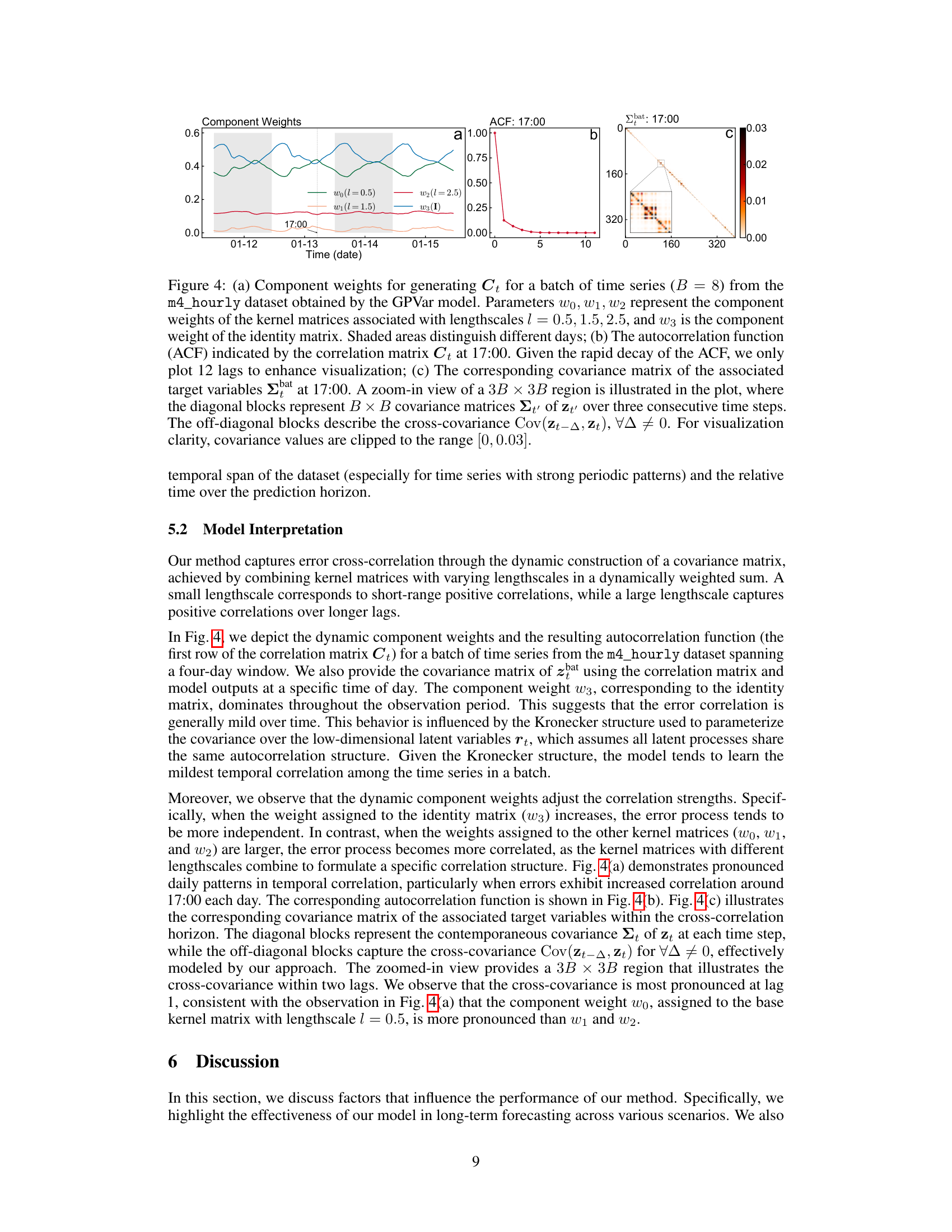
🔼 This figure shows the component weights used to generate the dynamic correlation matrix (Ct) at different time points, the autocorrelation function (ACF) of Ct at a specific time (17:00), and the corresponding covariance matrix of the time series variables at that time. The figure highlights the dynamic nature of the correlation structure and its relationship to the model parameters.
read the caption
Figure 4: (a) Component weights for generating Ct for a batch of time series (B = 8) from the m4_hourly dataset obtained by the GPVar model. Parameters wo, W1, W2 represent the component weights of the kernel matrices associated with lengthscales l = 0.5, 1.5, 2.5, and w3 is the component weight of the identity matrix. Shaded areas distinguish different days; (b) The autocorrelation function (ACF) indicated by the correlation matrix Ct at 17:00. Given the rapid decay of the ACF, we only plot 12 lags to enhance visualization; (c) The corresponding covariance matrix of the associated target variables Σbat at 17:00. A zoom-in view of a 3B × 3B region is illustrated in the plot, where the diagonal blocks represent B × B covariance matrices Σt of zt, over three consecutive time steps. The off-diagonal blocks describe the cross-covariance Cov(zt−∆, zt), ∀∆ ≠ 0. For visualization clarity, covariance values are clipped to the range [0, 0.03].

🔼 This figure visualizes the training and validation loss curves for the GPVar model, comparing the performance with and without the proposed method that incorporates time-dependent errors. The x-axis represents the training steps (time), and the y-axis shows the loss. Separate curves are plotted for training and validation loss, with and without the proposed method. This allows for a direct comparison of the impact of modeling temporal error correlations on the convergence and generalization performance of the model.
read the caption
Figure 5: Training loss/validation loss vs training time of the GPVar model. 'w/o' denotes methods without time-dependent errors, while 'w/' indicates our method.
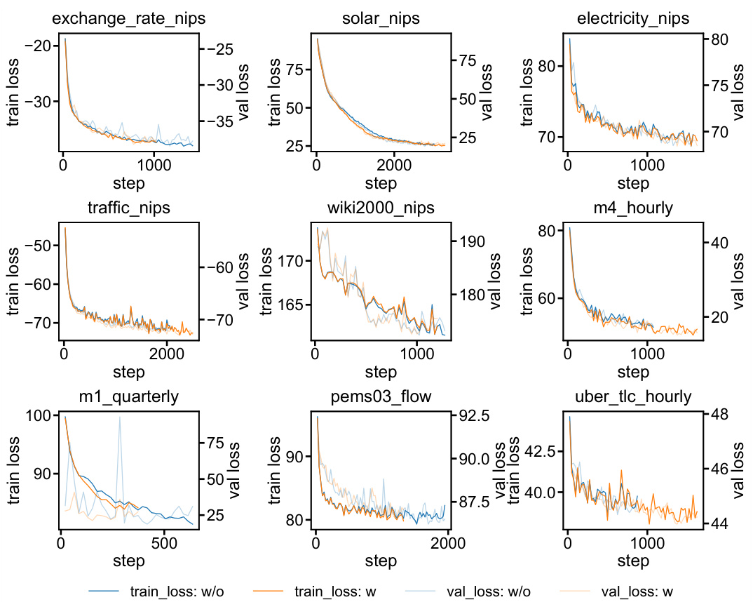
🔼 This figure compares the training and validation loss curves for the GPVar model with and without the proposed method for incorporating time-dependent errors. The x-axis represents the training steps, and the y-axis shows the loss values. Separate curves are plotted for training loss and validation loss for each model (with and without time-dependent errors). The figure helps to visualize the convergence speed and generalization performance of the models with and without the method.
read the caption
Figure 5: Training loss/validation loss vs training time of the GPVar model. 'w/o' denotes methods without time-dependent errors, while 'w/' indicates our method.

🔼 This figure shows how the number of time series used during prediction affects the performance of the proposed method and a baseline method (without time-dependent errors). The results are presented for several different datasets. The x-axis shows the number of time series in a batch during prediction, and the y-axis shows the CRPSsum, a metric to evaluate the accuracy of probabilistic forecasts. The lines represent the performance of the methods with and without the proposed method for modeling temporally correlated errors. It highlights that the benefit of including temporal error correlation diminishes when the number of time series is smaller than the batch size during training.
read the caption
Figure 7: The influence of the number of time series in a batch on the performance of inference. 'w/o' denotes methods without time-dependent errors, while 'w/' indicates our method. We only show some datasets here because the remaining datasets have fewer than B = 20 time series in the testing set.

🔼 This figure compares the autocorrelation function (ACF) of one-step-ahead prediction residuals obtained using GPVar with and without the proposed method for four time series from the solar dataset. The ACF measures the correlation between a time series and its lagged values. For each time series, two lines are shown: one for the model without the method (w/o), and one for the model with the proposed method (w/). The plots show that the proposed method reduces the autocorrelation in the residuals, indicating that it better captures and accounts for the temporal dependence in the data.
read the caption
Figure 8: ACF comparison of the one-step-ahead prediction residuals with and without our method. The results depict the prediction outcomes generated by GPVar for four time series in the solar dataset.

🔼 This figure compares the autocorrelation function (ACF) of the residuals from a one-step-ahead prediction model (GPVar) with and without the proposed method for four time series in the solar dataset. The ACF plots show the correlation of the residuals at different lags. Comparing the ‘w/o’ (without the method) and ‘w/’ (with the method) plots helps visualize how the proposed method affects the temporal correlation structure of the residuals, aiming for less autocorrelation.
read the caption
Figure 8: ACF comparison of the one-step-ahead prediction residuals with and without our method. The results depict the prediction outcomes generated by GPVar for four time series in the solar dataset.

🔼 This figure compares the autocorrelation function (ACF) plots of the one-step-ahead prediction residuals generated by GPVar model with and without the proposed method that incorporates temporally correlated errors. Four time series from the solar dataset are shown to illustrate the effectiveness of the method. The blue dots represent the ACF of residuals from the base model (without correlated errors), while the orange dots represent the ACF of residuals from the improved model. This visual comparison helps to demonstrate the reduction in autocorrelation achieved by the method.
read the caption
Figure 8: ACF comparison of the one-step-ahead prediction residuals with and without our method. The results depict the prediction outcomes generated by GPVar for four time series in the solar dataset.

🔼 This figure compares the autocorrelation function (ACF) plots of the one-step-ahead prediction residuals generated by the GPVar model, both with and without the proposed method for handling correlated errors. Four individual time series (A-D) are shown, each with two ACF plots (one for the model without and one for the model with the proposed method). The plots show how the proposed method effectively reduces the autocorrelation in prediction residuals across multiple time lags.
read the caption
Figure 8: ACF comparison of the one-step-ahead prediction residuals with and without our method. The results depict the prediction outcomes generated by GPVar for four time series in the solar dataset.
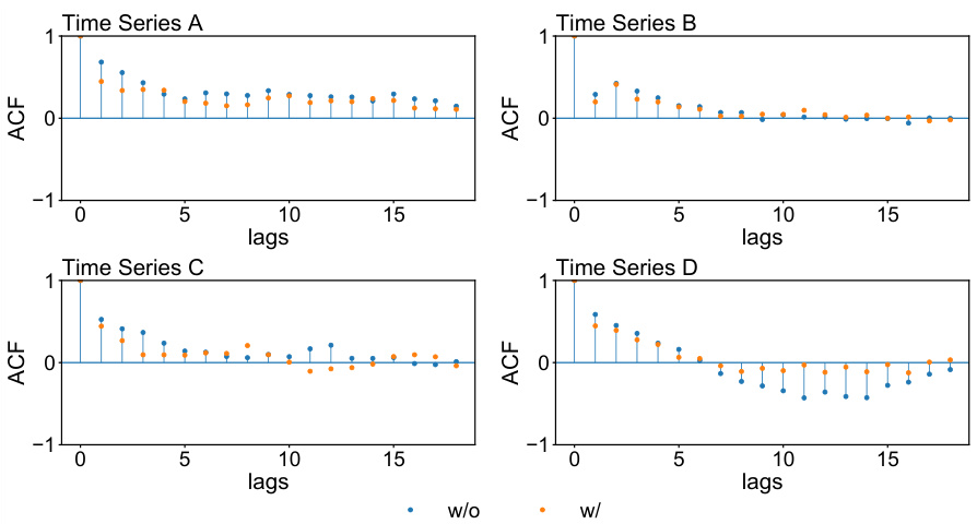
🔼 This figure compares the autocorrelation function (ACF) plots of the one-step-ahead prediction residuals obtained from the GPVar model with and without the proposed method. The analysis is performed on four different time series from the solar dataset. The plots show the autocorrelation of the residuals across multiple time lags. The comparison is designed to visually illustrate the impact of the proposed method in reducing the autocorrelation of the prediction residuals.
read the caption
Figure 8: ACF comparison of the one-step-ahead prediction residuals with and without our method. The results depict the prediction outcomes generated by GPVar for four time series in the solar dataset.

🔼 This figure compares the autocorrelation function (ACF) plots of the one-step-ahead prediction residuals generated by the GPVar model, with and without the proposed method for handling correlated errors. The results are shown for four different time series from the solar dataset. The ACF plots show the correlation of the residuals at different lags. A lag of 0 represents the correlation of the residuals with themselves, a lag of 1 represents the correlation between consecutive residuals, and so on. The comparison helps to visually assess the effectiveness of the method in reducing autocorrelation in the prediction residuals.
read the caption
Figure 8: ACF comparison of the one-step-ahead prediction residuals with and without our method. The results depict the prediction outcomes generated by GPVar for four time series in the solar dataset.

🔼 This figure compares the autocorrelation function (ACF) plots of prediction residuals for four different time series. The blue points represent the ACF of the residuals from the model without the proposed method for handling correlated errors, while the orange points show the ACF of the residuals from the model with the proposed method. The x-axis represents the lags (time steps), and the y-axis represents the ACF value. The plot illustrates how the proposed method reduces the autocorrelation in the prediction residuals across all four time series.
read the caption
Figure 8: ACF comparison of the one-step-ahead prediction residuals with and without our method. The results depict the prediction outcomes generated by GPVar for four time series in the solar dataset.
🔼 This figure shows the contemporaneous and cross-covariance matrices of prediction residuals. The contemporaneous covariance shows the correlation between different time series at the same time step. The cross-covariance shows the correlation between different time series at different time steps (lag 1, 2, and 3). The data used is from the m4_hourly dataset, and the covariance values are clipped to the range [0, 0.6] for better visualization.
read the caption
Figure 1: Contemporaneous covariance matrix Cov(ηt, ηt) and cross-covariance matrix Cov(ηt−∆, ηt), ∆ = 1,2,3, calculated based on the one-step-ahead prediction residuals of GP-Var on a batch of time series from the m4_hourly dataset. For visualization clarity, covariance are clipped to the range [0, 0.6].

🔼 This figure shows the empirical contemporaneous and cross-covariance matrices of prediction residuals from a probabilistic forecasting model (GPVar) applied to the m4_hourly dataset. The contemporaneous covariance matrix, Cov(ηt, ηt), displays the correlation between different time series at the same time step. The cross-covariance matrices, Cov(ηt−∆, ηt) for ∆ = 1, 2, 3, illustrate the correlation between residuals at different time lags (∆). The visualizations are clipped to highlight correlations between 0 and 0.6 for better clarity.
read the caption
Figure 1: Contemporaneous covariance matrix Cov(ηt, ηt) and cross-covariance matrix Cov(ηt−∆, ηt), ∆ = 1,2,3, calculated based on the one-step-ahead prediction residuals of GP-Var on a batch of time series from the m4_hourly dataset. For visualization clarity, covariance are clipped to the range [0, 0.6].
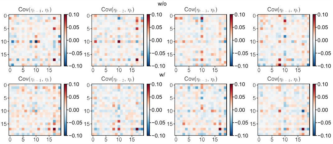
🔼 This figure compares the cross-correlation matrices of one-step ahead prediction residuals obtained from the GPVar model, with and without the proposed method for handling correlated errors. The matrices visualize the correlation between prediction residuals across different time lags and across different time series. Each subplot represents a specific time lag (1, 2, 3, and 4 steps). The color intensity represents the magnitude of cross-correlation; warmer colors indicate positive correlations, cooler colors indicate negative correlations, and lighter colors indicate near-zero correlation. The comparison aims to demonstrate the effectiveness of the proposed method in reducing cross-correlation.
read the caption
Figure 15: Cross-correlation comparison of the one-step-ahead prediction residuals with and without our method. The results depict the prediction outcomes generated by GPVar for four time series in the electricity dataset.

🔼 This figure compares the cross-correlation of residuals from a model trained with and without the proposed method for capturing cross-correlation in errors. It shows the cross-covariance matrices Cov(ηt−∆, ηt) for ∆ = 1, 2, 3, 4, where ηt represents the prediction residuals at time t. The top row shows the results when the model does not account for cross-correlation (w/o), while the bottom row shows the results when the model does account for cross-correlation (w/). The color scale represents the correlation strength; warmer colors indicate stronger positive correlation, and cooler colors indicate stronger negative correlation. The visual comparison aims to illustrate how the proposed method reduces cross-correlation among the residuals.
read the caption
Figure 15: Cross-correlation comparison of the one-step-ahead prediction residuals with and without our method. The results depict the prediction outcomes generated by GPVar for four time series in the electricity dataset.

🔼 This figure compares the cross-correlation of one-step-ahead prediction residuals using GPVAR with and without the proposed method to model correlated errors. Four different time series are shown (A, B, C, D). Each subplot shows the cross-covariance between residuals at time t and residuals at times t-1, t-2, t-3, and t-4. The color scale represents the correlation strength. The results indicate a reduction in cross-correlation after applying the proposed method.
read the caption
Figure 15: Cross-correlation comparison of the one-step-ahead prediction residuals with and without our method. The results depict the prediction outcomes generated by GPVar for four time series in the electricity dataset.

🔼 This figure compares the cross-correlation of residuals from the GPVar model with and without the proposed method for four time series in the electricity dataset. Specifically, it visualizes the cross-covariance matrices Cov(ηt−Δ, ηt), where Δ represents the lag (1, 2, 3, 4 steps) and ηt represents the residuals at time step t. The comparison shows that the proposed method effectively reduces cross-correlations in the residuals.
read the caption
Figure 15: Cross-correlation comparison of the one-step-ahead prediction residuals with and without our method. The results depict the prediction outcomes generated by GPVar for four time series in the electricity dataset.

🔼 This figure shows the empirical contemporaneous covariance matrix and cross-covariance matrices of prediction residuals from a multivariate time series model (GPVar) applied to the m4_hourly dataset. The contemporaneous covariance (Cov(ηt, ηt)) shows the correlation between different time series at the same time step. The cross-covariance matrices (Cov(ηt−∆, ηt) for ∆ = 1,2,3) show the correlation between errors at different time lags. The covariance values are clipped to a range [0,0.6] for better visualization.
read the caption
Figure 1: Contemporaneous covariance matrix Cov(ηt, ηt) and cross-covariance matrix Cov(ηt−∆, ηt), ∆ = 1,2,3, calculated based on the one-step-ahead prediction residuals of GP-Var on a batch of time series from the m4_hourly dataset. For visualization clarity, covariance are clipped to the range [0, 0.6].
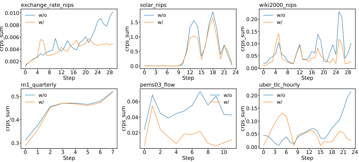
🔼 This figure compares the step-wise CRPSsum accuracy of the GPVar model with and without the proposed method for modeling correlated errors. The x-axis represents the forecast steps, and the y-axis shows the CRPSsum. Separate lines are shown for each dataset, comparing the model trained without considering temporal error correlations (‘w/o’) against the model trained with the proposed method (‘w/’). The results demonstrate that modeling time-dependent errors generally leads to improved accuracy, especially in the earlier forecast steps. Note that the improvement varies across datasets and may decrease or increase at later steps, likely influenced by the dataset’s characteristics such as seasonality and data variability.
read the caption
Figure 21: Step-wise CRPSsum accuracy of GPVar. “w/o” denotes methods without time-dependent errors, while “w/” indicates our method.
🔼 This figure shows the contemporaneous and cross-covariance matrices of prediction residuals from a multivariate autoregressive model. The contemporaneous covariance shows the correlation between errors at the same time step across different time series. The cross-covariance matrices (for lags 1, 2, and 3) depict the correlation between errors at different time steps. This visualization highlights the presence of both contemporaneous and temporal dependencies in the model’s residuals, which are usually ignored by simpler models for scalability reasons. The data used is from the m4_hourly dataset.
read the caption
Figure 1: Contemporaneous covariance matrix Cov(ηt, ηt) and cross-covariance matrix Cov(ηt−∆, ηt), ∆ = 1,2,3, calculated based on the one-step-ahead prediction residuals of GP-Var on a batch of time series from the m4_hourly dataset. For visualization clarity, covariance are clipped to the range [0, 0.6].
🔼 This figure shows the contemporaneous covariance matrix and cross-covariance matrices of prediction residuals from the GPVar model applied to the m4_hourly dataset. It visually demonstrates the temporal dependence in the residuals, which violates the common assumption of temporal independence in many time series models. The covariance matrices show correlations between residuals at different time steps (cross-covariance), indicating the presence of autocorrelation and cross-lag correlation in the errors.
read the caption
Figure 1: Contemporaneous covariance matrix Cov(nt, nt) and cross-covariance matrix Cov(nt−∆, ηt), ∆ = 1,2,3, calculated based on the one-step-ahead prediction residuals of GP-Var on a batch of time series from the m4_hourly dataset. For visualization clarity, covariance are clipped to the range [0, 0.6].

🔼 This figure shows an empirical example of the proposed method for learning cross-correlation in multivariate probabilistic forecasting models. It visualizes the component weights for generating the dynamic correlation matrix Ct (part a), the autocorrelation function (ACF) of Ct at a specific time (part b), and the corresponding covariance matrix of the time series variables at that time (part c). The figure demonstrates how the model captures dynamic correlation patterns and generates a time-varying covariance matrix for improving predictive accuracy.
read the caption
Figure 4: (a) Component weights for generating Ct for a batch of time series (B = 8) from the m4_hourly dataset obtained by the GPVar model. Parameters wo, W1, W2 represent the component weights of the kernel matrices associated with lengthscales l = 0.5, 1.5, 2.5, and w3 is the component weight of the identity matrix. Shaded areas distinguish different days; (b) The autocorrelation function (ACF) indicated by the correlation matrix Ct at 17:00. Given the rapid decay of the ACF, we only plot 12 lags to enhance visualization; (c) The corresponding covariance matrix of the associated target variables Et at 17:00. A zoom-in view of a 3B × 3B region is illustrated in the plot, where the diagonal blocks represent B × B covariance matrices Et of zł, over three consecutive time steps. The off-diagonal blocks describe the cross-covariance Cov(Zt−∆, Zt), ∀∆ ≠ 0. For visualization clarity, covariance values are clipped to the range [0, 0.03].

🔼 This figure shows the contemporaneous and cross-covariance matrices of prediction residuals obtained from a GPVar model trained on the m4_hourly dataset. The contemporaneous covariance matrix, Cov(nt, nt), displays the correlation between residuals at the same time step. The cross-covariance matrices, Cov(nt−∆, ηt) for ∆ = 1, 2, and 3, illustrate the correlation between residuals at different time steps (lags). The visualization uses a color scale to represent the covariance values, ranging from negative to positive correlation. The values are clipped for clarity.
read the caption
Figure 1: Contemporaneous covariance matrix Cov(nt, nt) and cross-covariance matrix Cov(nt−∆, ηt), ∆ = 1,2,3, calculated based on the one-step-ahead prediction residuals of GP-Var on a batch of time series from the m4_hourly dataset. For visualization clarity, covariance are clipped to the range [−0.6, 0.6].
🔼 This figure shows the contemporaneous and cross-covariance matrices of prediction residuals from a multivariate time series model (GP-Var) applied to the m4_hourly dataset. The contemporaneous covariance (Cov(ηt, ηt)) represents the correlation between errors at the same time step, while the cross-covariance matrices (Cov(ηt−∆, ηt) for ∆ = 1, 2, 3) show correlations between errors at different time lags. The visualization helps to illustrate the presence of temporal dependencies in the residuals, which are not accounted for in many time series models.
read the caption
Figure 1: Contemporaneous covariance matrix Cov(ηt, ηt) and cross-covariance matrix Cov(ηt−∆, ηt), ∆ = 1,2,3, calculated based on the one-step-ahead prediction residuals of GP-Var on a batch of time series from the m4_hourly dataset. For visualization clarity, covariance are clipped to the range [−0.6, 0.6].

🔼 This figure shows the contemporaneous and cross-covariance matrices of prediction residuals. The contemporaneous covariance matrix Cov(nt, nt) displays the correlation between errors at the same time step. The cross-covariance matrices Cov(nt−∆, ηt) show the correlation between errors at different time steps (lags ∆ = 1, 2, 3). The data used is from the m4_hourly dataset, and the covariances are capped at 0.6 for better visualization.
read the caption
Figure 1: Contemporaneous covariance matrix Cov(nt, nt) and cross-covariance matrix Cov(nt−∆, ηt), ∆ = 1,2,3, calculated based on the one-step-ahead prediction residuals of GP-Var on a batch of time series from the m4_hourly dataset. For visualization clarity, covariance are clipped to the range [0, 0.6].
🔼 This figure displays the contemporaneous and cross-covariance matrices calculated from the prediction residuals of a GPVAR model trained on the m4_hourly dataset. The contemporaneous covariance matrix shows the covariance between the errors at the same time step. The cross-covariance matrices show the covariance between the errors at different time steps (lags 1, 2, and 3). The covariance values are clipped to the range [0, 0.6] for better visualization.
read the caption
Figure 1: Contemporaneous covariance matrix Cov(nt, nt) and cross-covariance matrix Cov(nt−∆, ηt), ∆ = 1,2,3, calculated based on the one-step-ahead prediction residuals of GP-Var on a batch of time series from the m4_hourly dataset. For visualization clarity, covariance are clipped to the range [0, 0.6].
🔼 This figure illustrates how the proposed method incorporates temporal dependencies in the latent variable within a batch to address cross-correlated errors in multivariate probabilistic forecasting. Unlike the traditional approach, which models the likelihood independently at each time step, the proposed method models dependencies over an extended temporal window, enhancing the capture of cross-correlation. This figure uses RNN as an example, but the concept applies to other autoregressive models as well. The model parameters are shared across all dimensions, making the method computationally efficient.
read the caption
Figure 3: Illustration of the training process. Following [3], time series dimensions are randomly sampled, and the base model (e.g., RNNs) is unrolled for each dimension individually (e.g., 1, 2, 4, followed by 1, 3, 4 as depicted). The model parameters are shared across all time series dimensions. A batch of time series variables zhat contains time series vectors zł covering time steps from t − D+1 to t. In contrast to [3], our approach explicitly models dependencies over the extended temporal window from t − D + 1 to t during training.
More on tables

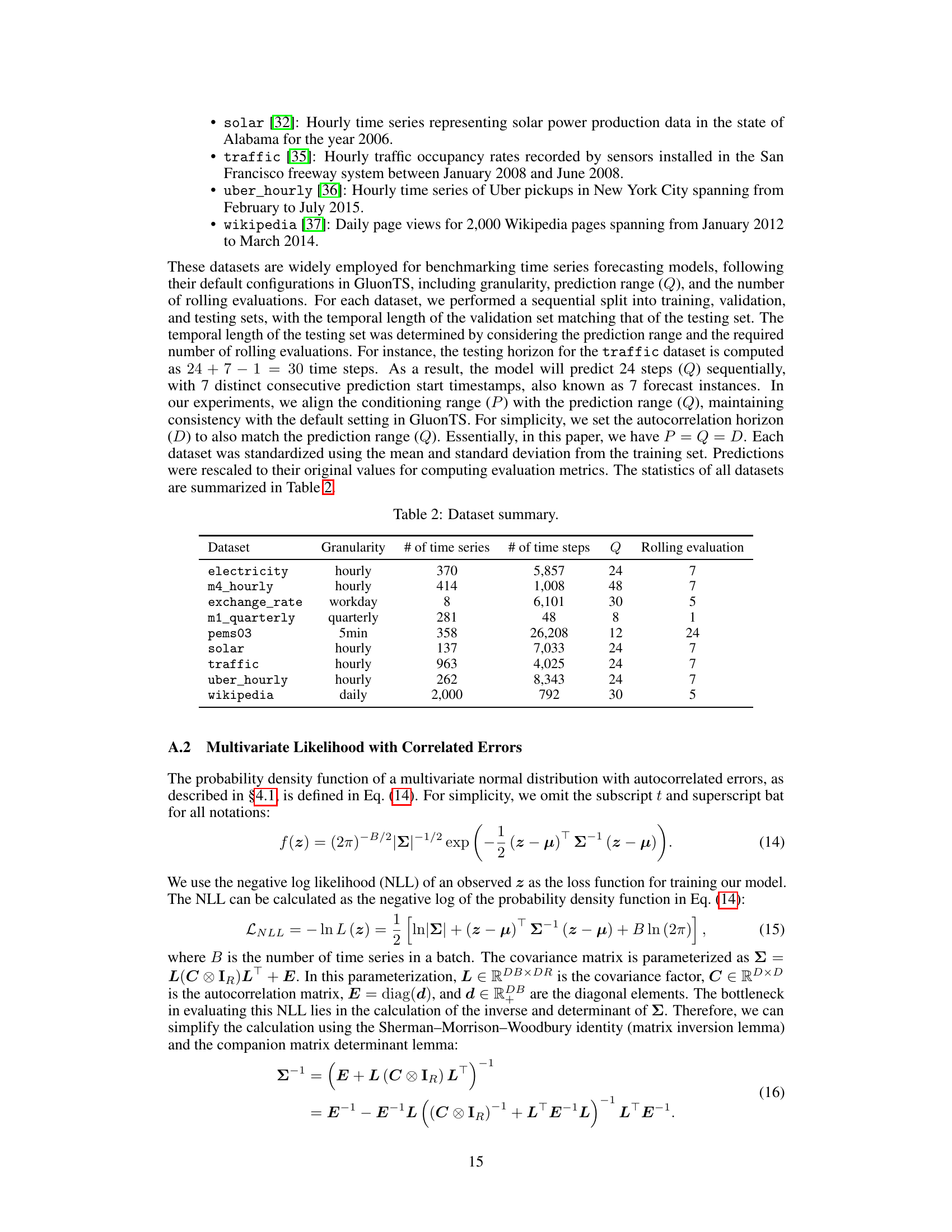
🔼 This table summarizes the characteristics of the nine datasets used in the experiments. For each dataset, it lists the granularity of the time series data (hourly, daily, etc.), the total number of time series, the total number of time steps in the dataset, the prediction range (Q) used for forecasting, and the number of rolling evaluations performed for each time series.
read the caption
Table 2: Dataset summary.

🔼 This table lists the hyperparameters used in the experiments. It shows which hyperparameters were fixed to a certain value and which hyperparameters were tuned by searching over a range of values. The hyperparameters being tuned include the learning rate, the number of LSTM cells or the dimension of the transformer model, the number of LSTM layers or transformer decoder layers, the number of attention heads in the transformer, the rank of the covariance matrix, the sampling dimension, the dropout rate, and the batch size.
read the caption
Table 3: Hyperparameters values that are fixed or searched over a range during hyperparameter tuning.

🔼 This table lists the hyperparameters used in the experiments. It shows which hyperparameters were fixed and which hyperparameters had their values searched over a range during the hyperparameter tuning phase. The table is valuable because it helps readers understand how the authors arrived at the model configurations they used in their experiments, including choices about learning rates, the number of layers in recurrent networks, the size of the model, and various regularization parameters.
read the caption
Table 3: Hyperparameters values that are fixed or searched over a range during hyperparameter tuning.

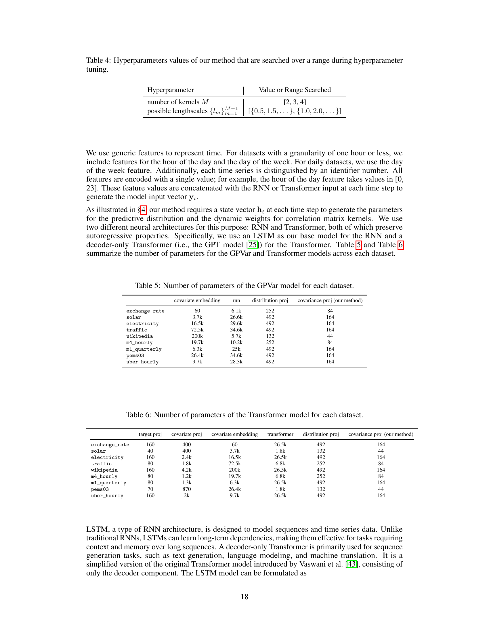
🔼 This table shows the number of parameters used in the GPVar model for each dataset, broken down into the number of parameters used for covariate embedding, RNN, distribution projection, and covariance projection (the authors’ method). It helps illustrate the model’s complexity and parameter efficiency.
read the caption
Table 5: Number of parameters of the GPVar model for each dataset.

🔼 This table shows the number of parameters for different components of the Transformer model used in the paper for each dataset. The components include those for the target projection, covariate projection, covariate embedding, the Transformer itself, the distribution projection, and finally, the covariance projection using the authors’ method. The table is useful to understand the model’s complexity and how the proposed method scales across different datasets.
read the caption
Table 6: Number of parameters of the Transformer model for each dataset.

🔼 This table presents a comparison of the Continuous Ranked Probability Score sum (CRPSsum) for various time series forecasting models. The CRPSsum metric measures the accuracy of probabilistic forecasts. The table compares models trained without considering time-dependent errors (‘w/o’) against those that do (‘w/’). Bold values highlight instances where incorporating time-dependent errors resulted in better performance. The results are averaged across 10 runs for each model to account for randomness.
read the caption
Table 1: CRPSsum accuracy comparison. 'w/o' denotes methods without time-dependent errors, while 'w/' indicates our method. Bold values show models with time-dependent errors performing better. Mean and standard deviation are obtained from 10 runs of each model.

🔼 This table presents a comparison of the Continuous Ranked Probability Score (CRPS) for various time series forecasting models. It compares models that do not consider temporal error correlations (‘w/o’) to those that do (‘w/’). The results are averaged across 10 runs for each model. Bold values highlight cases where considering time-dependent errors leads to improved accuracy (lower CRPS).
read the caption
Table 1: CRPSsum accuracy comparison. 'w/o' denotes methods without time-dependent errors, while 'w/' indicates our method. Bold values show models with time-dependent errors performing better. Mean and standard deviation are obtained from 10 runs of each model.

🔼 This table presents a comparison of the Continuous Ranked Probability Score sum (CRPSsum) for various time series forecasting models. The models are categorized into two groups: those without time-dependent errors (‘w/o’) and those with time-dependent errors (‘w/’). The table shows the CRPSsum values (with standard deviations) for each model across eight different datasets (exchange_rate, solar, electricity, traffic, wiki, m4_hourly, m1_quarterly, pems03, uber_hourly). Bold values indicate cases where models using the proposed method for incorporating time-dependent errors show improved accuracy. The average relative improvement in CRPSsum is also provided for both GPVar and Transformer models.
read the caption
Table 1: CRPSsum accuracy comparison. 'w/o' denotes methods without time-dependent errors, while 'w/' indicates our method. Bold values show models with time-dependent errors performing better. Mean and standard deviation are obtained from 10 runs of each model.

🔼 This table presents a comparison of the Continuous Ranked Probability Score sum (CRPSsum) achieved by various models on multiple datasets. It compares models trained without considering time-dependent errors (‘w/o’) to those trained with the proposed method for incorporating correlated errors (‘w/’). The bold values highlight instances where including time-dependent errors leads to improved accuracy. The average relative improvement is reported, showing the effectiveness of the proposed method.
read the caption
Table 1: CRPSsum accuracy comparison. 'w/o' denotes methods without time-dependent errors, while 'w/' indicates our method. Bold values show models with time-dependent errors performing better. Mean and standard deviation are obtained from 10 runs of each model.

🔼 This table presents a comparison of the continuous ranked probability score (CRPS) sum for various multivariate time series forecasting models. The ‘w/o’ column represents models without considering the time-dependence of errors, while the ‘w/’ column represents models incorporating the proposed method for handling correlated errors. Bold values indicate instances where the proposed method (w/) outperforms the baseline (w/o). The results are averaged over ten runs for each model to provide statistical significance.
read the caption
Table 1: CRPSsum accuracy comparison. 'w/o' denotes methods without time-dependent errors, while 'w/' indicates our method. Bold values show models with time-dependent errors performing better. Mean and standard deviation are obtained from 10 runs of each model.

🔼 This table compares the Continuous Ranked Probability Score (CRPS) sum, a metric for evaluating probabilistic forecasting accuracy, across multiple models and datasets. It contrasts models trained without considering time-dependent errors (‘w/o’) against those that do incorporate such errors using the proposed method (‘w/’). The lower the CRPSsum value, the better the model’s performance. Bold values highlight cases where incorporating time-dependent errors significantly improved the model’s predictive ability. The mean and standard deviation were calculated over ten runs for each model to provide a reliable estimate of performance.
read the caption
Table 1: CRPSsum accuracy comparison. 'w/o' denotes methods without time-dependent errors, while 'w/' indicates our method. Bold values show models with time-dependent errors performing better. Mean and standard deviation are obtained from 10 runs of each model.

🔼 This table presents a comparison of the Continuous Ranked Probability Score (CRPS) sum for various time series forecasting models. It contrasts models that do not account for time-dependent errors (‘w/o’) against models that incorporate the proposed method for handling such errors (‘w/’). The bold values highlight instances where incorporating time-dependent errors leads to improved accuracy. The results represent the mean and standard deviation from 10 independent runs for each model and dataset.
read the caption
Table 1: CRPSsum accuracy comparison. 'w/o' denotes methods without time-dependent errors, while 'w/' indicates our method. Bold values show models with time-dependent errors performing better. Mean and standard deviation are obtained from 10 runs of each model.

🔼 This table presents a comparison of the Continuous Ranked Probability Score (CRPS) sum across multiple time series forecasting models. It compares models trained without considering time-dependent errors (‘w/o’) against models incorporating the proposed method for handling correlated errors (‘w/’). The bold values highlight instances where the method incorporating time-dependent errors shows improved accuracy. Results are averaged over 10 independent runs for each model.
read the caption
Table 1: CRPSsum accuracy comparison. 'w/o' denotes methods without time-dependent errors, while 'w/' indicates our method. Bold values show models with time-dependent errors performing better. Mean and standard deviation are obtained from 10 runs of each model.

🔼 This table compares the Continuous Ranked Probability Score (CRPS) for different probabilistic forecasting models with and without the proposed method for handling correlated errors. The models are evaluated on multiple real-world datasets, and CRPS is calculated for both Gaussian-distributed and t-distributed errors. The results show the improvements gained using the proposed method to model the correlation structure of errors across multiple time steps.
read the caption
Table 15: CRPSsum accuracy comparison. 'w/o' denotes methods without time-dependent errors, while 'w/' indicates our method. Bold values show models with time-dependent errors performing better. Mean and standard deviation are obtained from 10 runs of each model. 'N/A' indicates that the model could not be properly fitted.
Full paper#

