TL;DR#
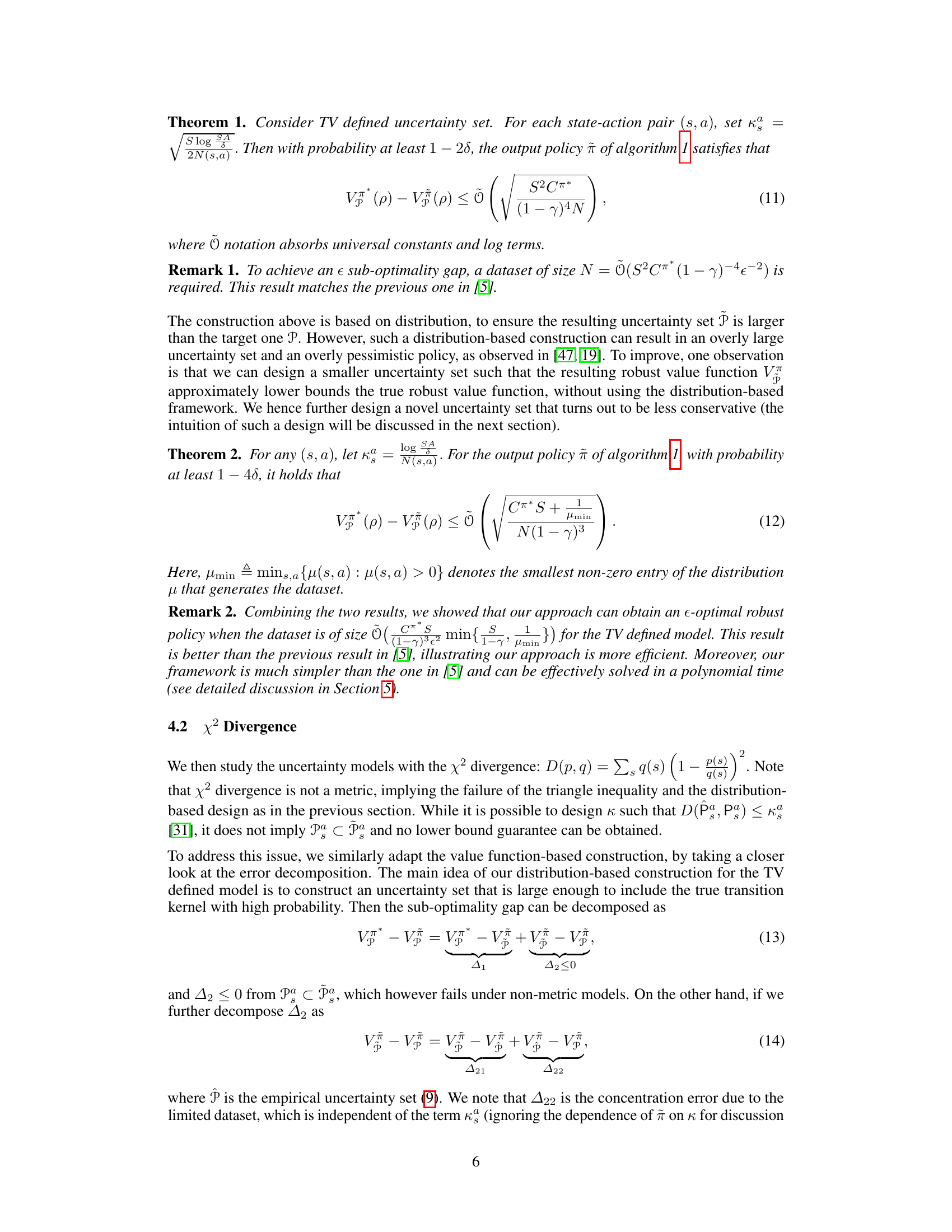
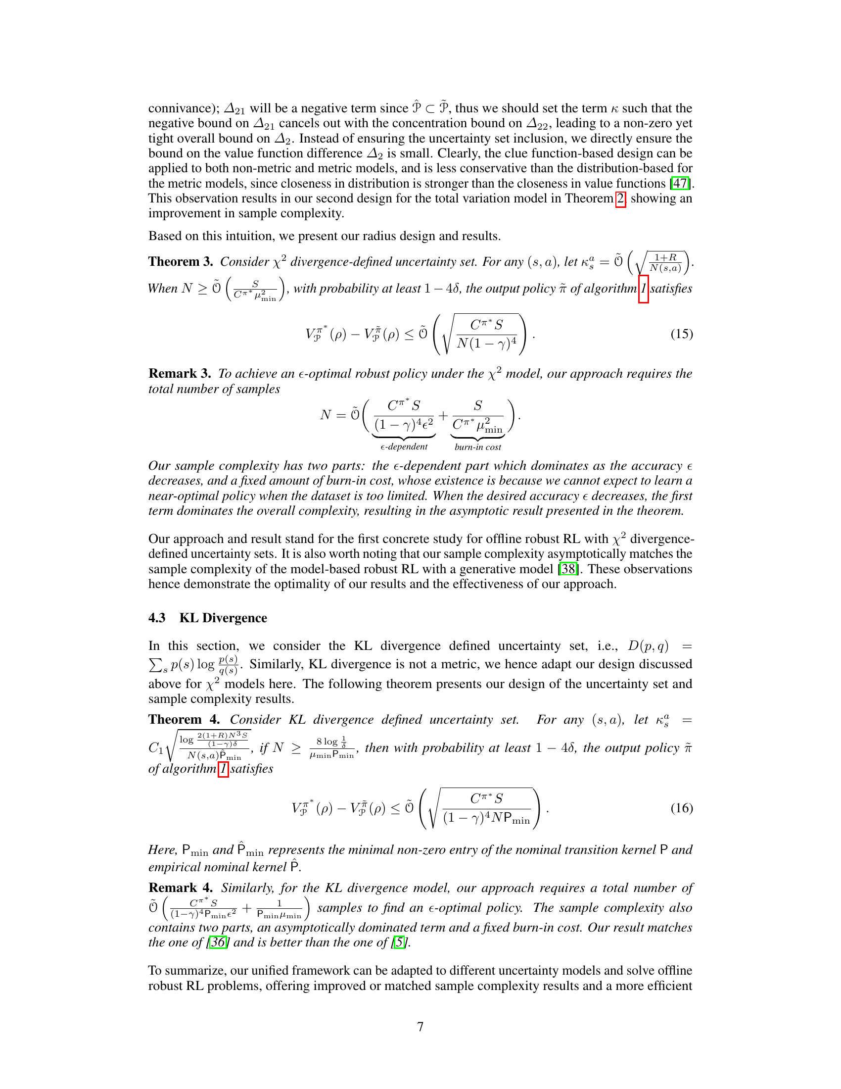
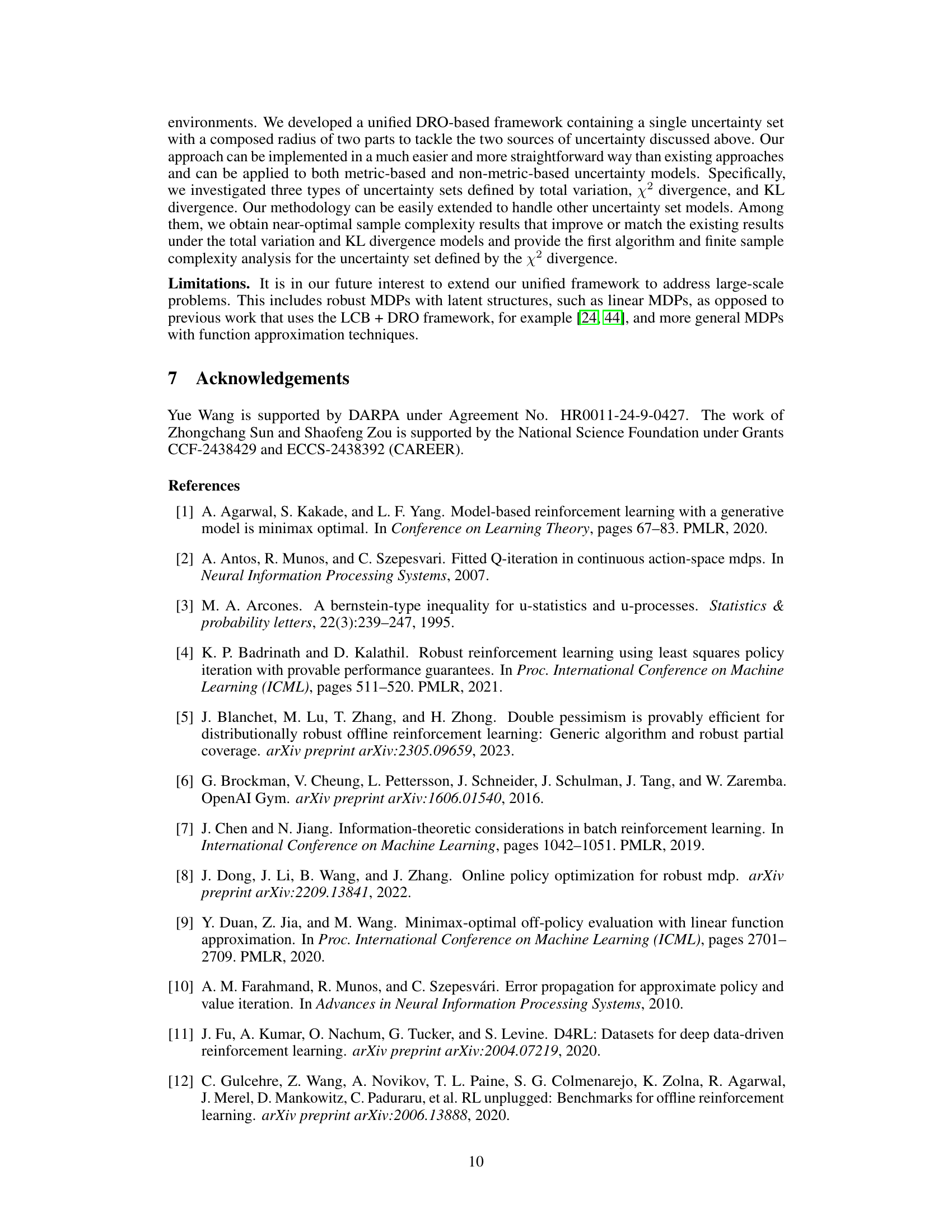
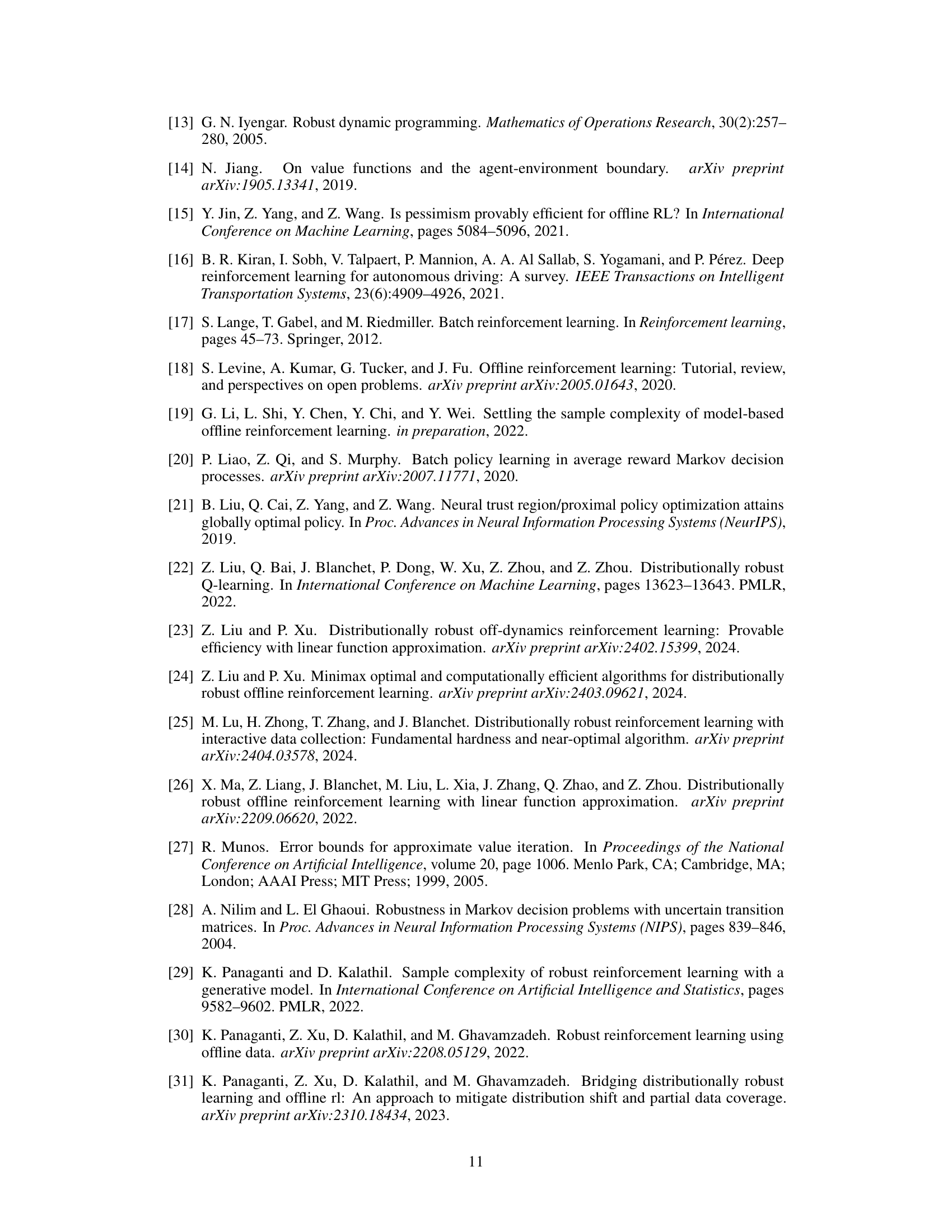
Offline reinforcement learning (RL) aims to learn optimal policies from pre-collected datasets, avoiding costly and risky online interactions. However, real-world offline RL faces two major challenges: inaccurate model estimation due to limited data and performance degradation from model mismatch between the training and deployment environments. Existing methods often tackle these issues separately, leading to redundancy or complexity.
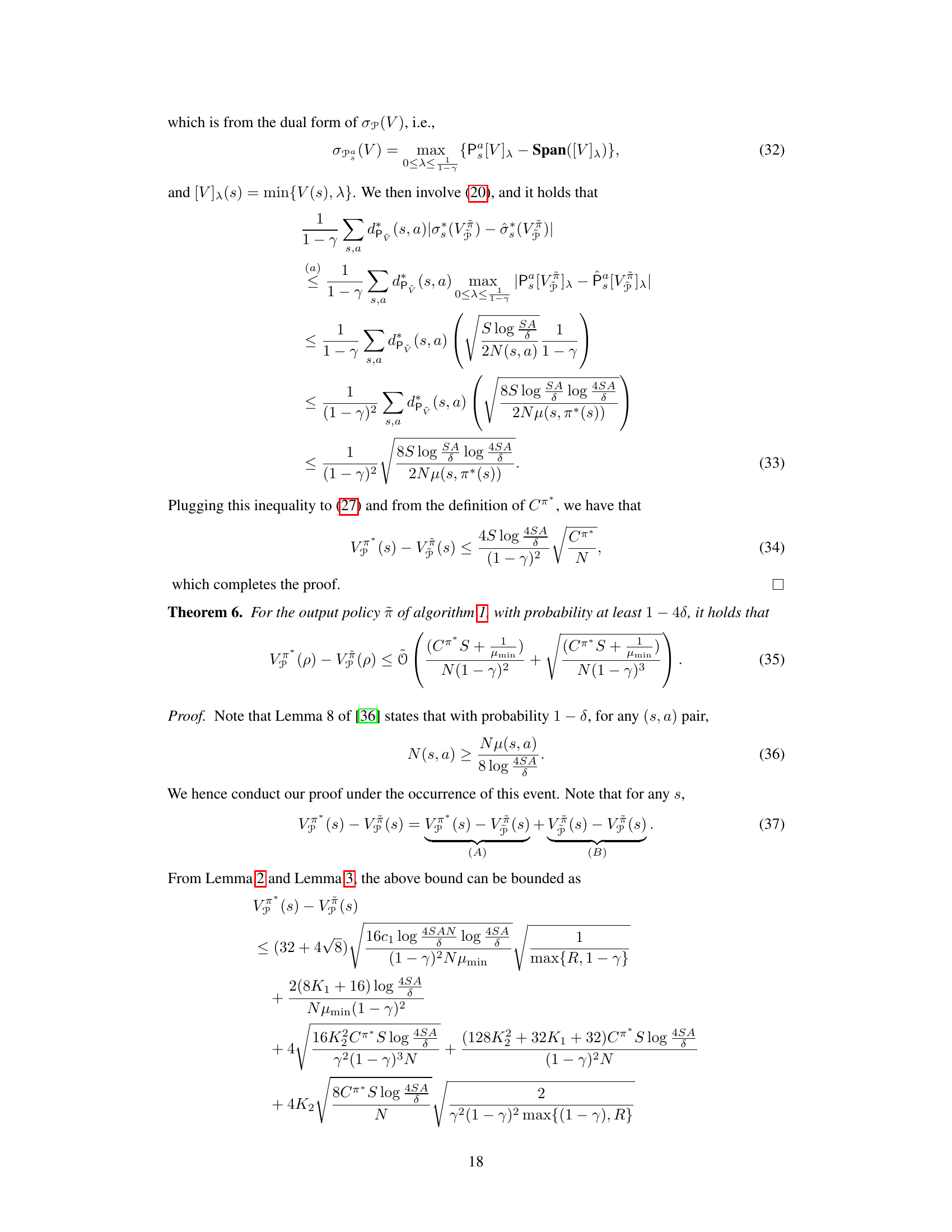
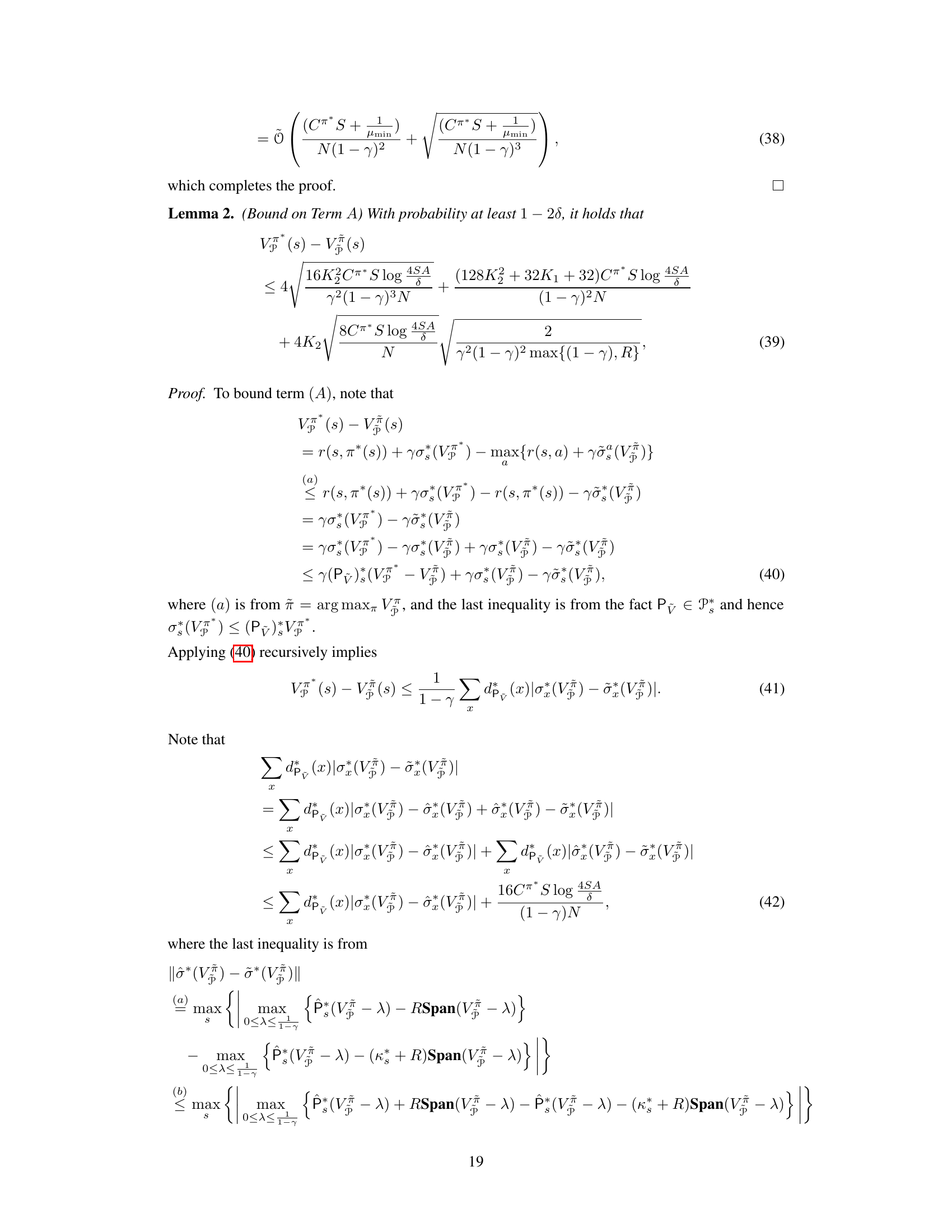
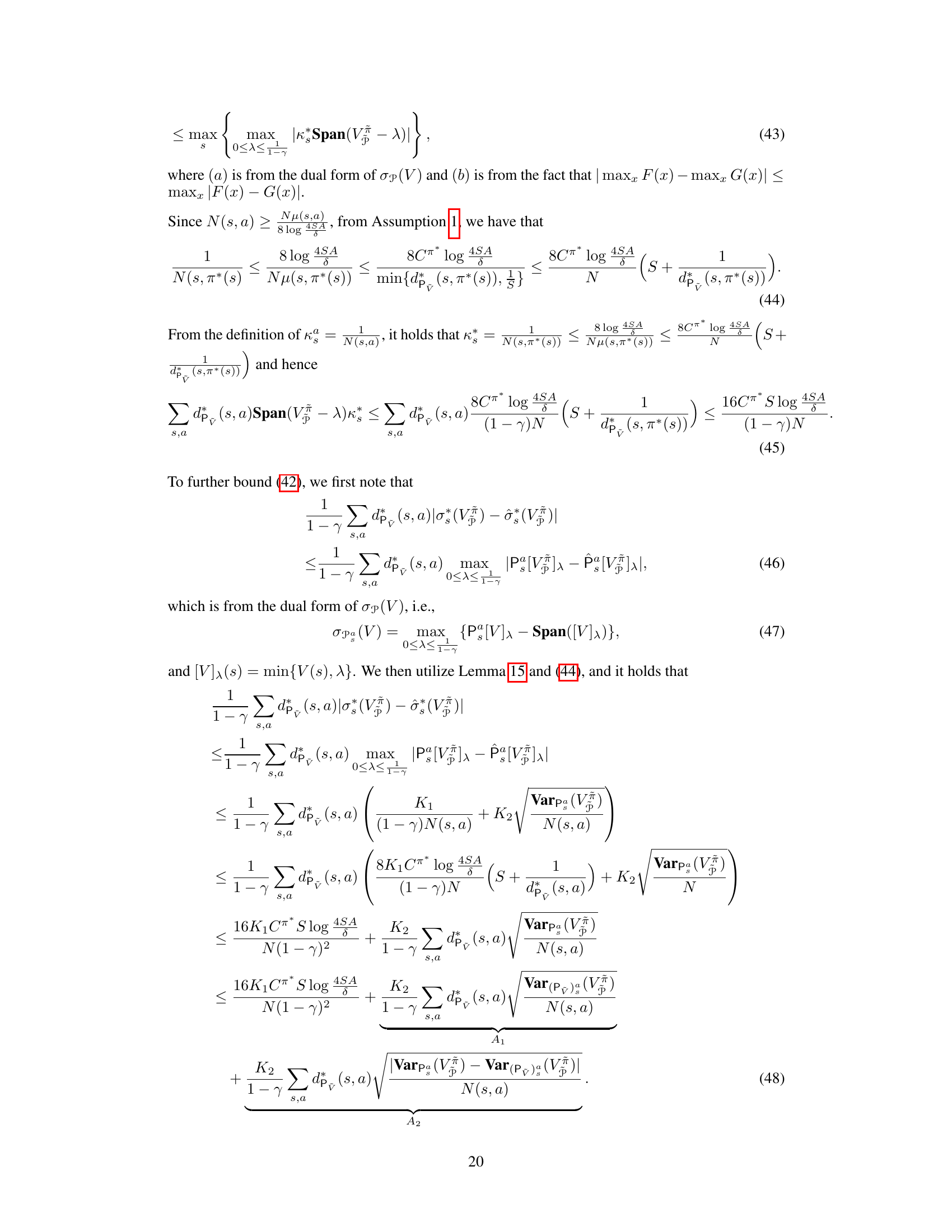
This research introduces a novel unified framework that integrates both principles of pessimism into a single robust Markov Decision Process (MDP). This unified approach addresses both data sparsity and model mismatch simultaneously by carefully constructing a robust MDP with a single uncertainty set. The results demonstrate near-optimal sub-optimality gap under the target environment across three uncertainty models: total variation, chi-squared divergence, and KL divergence. These findings improve upon or match state-of-the-art performance for total variation and KL divergence and provide the first result for chi-squared divergence.
Key Takeaways#
Why does it matter?#
This paper is crucial because it presents a unified framework for offline reinforcement learning that tackles both data sparsity and model mismatch, two major challenges hindering real-world applications. This work offers improved theoretical guarantees and practical efficiency, opening new avenues for robust offline RL research.
Visual Insights#
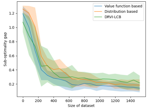
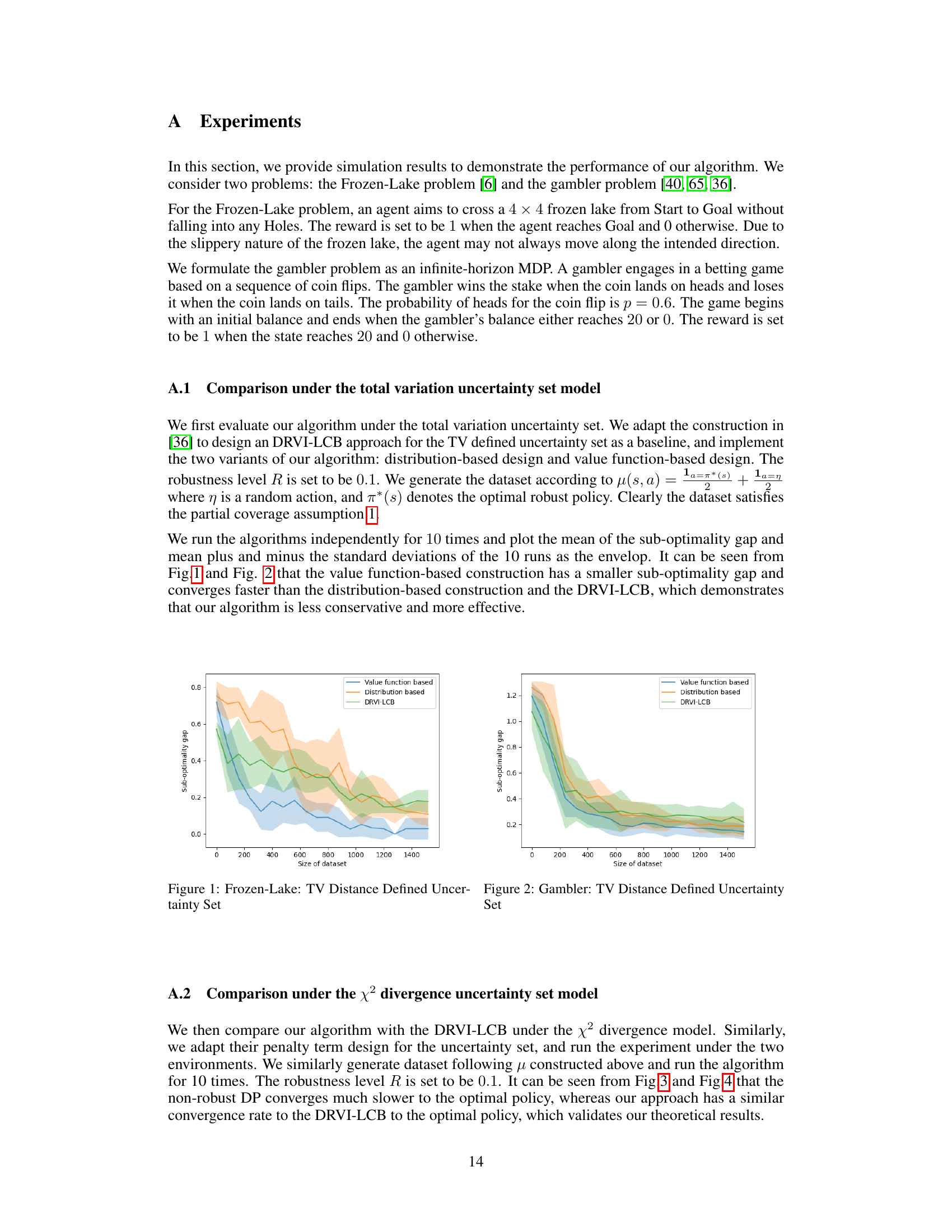
🔼 The figure shows the performance comparison of three algorithms under the total variation uncertainty model in the Frozen Lake environment. The x-axis represents the size of the dataset, and the y-axis represents the sub-optimality gap. The three algorithms compared are: value function based, distribution based, and DRVI-LCB. The shaded area around each line represents the standard deviation across multiple runs. The figure demonstrates that the value function based approach outperforms the other two in terms of both convergence speed and final sub-optimality gap.
read the caption
Figure 1: Frozen-Lake: TV Distance Defined Uncertainty Set

🔼 This table compares the sample complexities of three different offline reinforcement learning (RL) methods under three different divergence measures (Total Variation, Chi-squared, and Kullback-Leibler). It highlights the improvements achieved by the proposed unified framework in terms of sample complexity compared to previous state-of-the-art methods. The table showcases the trade-off between the complexity of handling data sparsity and model mismatch.
read the caption
Table 1: Comparison with related works on offline RL under model mismatch. In [5], Cob is the robust partial coverage coefficient [5], which is similar to Cπ*, and the exp((1 – γ)−1) term can be eliminated with an additional cost on Pmin−1 and μmin−1.
In-depth insights#
Offline RL’s Challenge#
Offline reinforcement learning (RL) presents unique challenges stemming from the inherent limitations of using a pre-collected dataset. Data sparsity, where the dataset lacks sufficient coverage of state-action pairs, hinders accurate model learning and optimal policy discovery. This leads to poor generalization and suboptimal performance in unseen situations. Furthermore, model mismatch arises when the offline dataset’s environment differs from the target deployment environment. This discrepancy, caused by environmental changes or inconsistencies in data collection, degrades the learned policy’s effectiveness in the real-world. Addressing these challenges requires innovative techniques. Pessimistic approaches that account for uncertainty are crucial for robust offline RL performance. These techniques incorporate caution in regions of limited data or potential model inaccuracies, thus improving generalization and mitigating the risks associated with data sparsity and model mismatch.
Pessimism Principle#
The “Pessimism Principle” in offline reinforcement learning (RL) addresses the challenge of uncertainty stemming from limited and potentially biased datasets. It acknowledges the inherent risk of overestimating the value of actions based on limited observations, particularly in offline settings where the agent lacks the opportunity for extensive exploration. The core idea is to introduce a degree of pessimism in the learning process, essentially underestimating the reward potential of actions that are poorly represented in the dataset. This avoids overly optimistic policies that may perform poorly during deployment due to data sparsity or model mismatch. The principle manifests in various ways, such as using lower confidence bounds on reward estimates or distributionally robust optimization. The careful balance between pessimism and optimism is crucial for ensuring both safety (avoiding catastrophic actions) and good performance. Methods incorporating the pessimism principle often aim to provide theoretical guarantees on the performance gap between a learned policy and an optimal one, considering uncertainty in the model and data. Therefore, it plays a critical role in developing reliable offline RL algorithms that can be deployed in real-world scenarios.
Unified Robust MDP#
A Unified Robust MDP framework is a significant advancement in offline reinforcement learning (RL), offering a principled way to address the critical challenges of model mismatch and data sparsity. By integrating both principles of pessimism into a single robust Markov Decision Process (MDP), it avoids the redundancy and complexity of separate approaches. This unified framework is crucial because offline RL relies on pre-collected data, which might not perfectly represent the deployment environment, and data scarcity limits reliable model estimations. A core strength lies in the formulation’s ability to tackle these issues concurrently through a single uncertainty set, leveraging distributional robustness to handle model mismatch and incorporating a data-dependent penalization term to mitigate data sparsity. This provides theoretical guarantees and improved performance compared to existing methods, offering a streamlined and theoretically sound methodology for real-world applications.
Theoretical Guarantee#
A theoretical guarantee section in a research paper provides a rigorous mathematical analysis to support the claims made by the paper. It aims to establish that the proposed method or algorithm will achieve a certain level of performance, under specific conditions. This is crucial for establishing credibility and reliability, especially when empirical results alone may be insufficient due to factors like limited experimental settings or variations in data. A strong theoretical guarantee often involves deriving bounds or rates of convergence that quantify the algorithm’s performance relative to some optimal solution. The strength of the guarantee depends on the tightness of the bounds and the generality of the underlying assumptions. Assumptions are vital to defining the scope and applicability of the guarantee, and limitations of these assumptions should also be clearly stated. The methods used for deriving the guarantee might include techniques from probability theory, statistics, information theory, and optimization theory. A rigorous proof is often needed to verify the validity of the guarantee.
Future Works#
The “Future Works” section of this research paper presents exciting avenues for extending the current research on offline reinforcement learning under model mismatch. A key area for future exploration is scaling the algorithms to handle larger, more complex real-world problems. This includes adapting the techniques to latent-structured models, such as linear MDPs, which are more realistic and efficient representations for high-dimensional environments. Another crucial direction is to investigate more general function approximation methods, moving beyond the limitations of tabular settings to handle continuous state and action spaces. Furthermore, robustness to more general forms of model mismatch needs to be explored, potentially involving methods from domain adaptation or transfer learning. Investigating alternative uncertainty set models or refining the radius design is vital to enhance both practical efficiency and theoretical guarantees. Finally, a comprehensive empirical evaluation on various benchmark tasks would strengthen the findings and showcase the practical applicability of this approach.
More visual insights#
More on figures
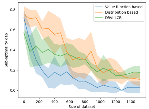
🔼 The figure shows the comparison of three algorithms under the total variation uncertainty set model on the Frozen-Lake problem. The three algorithms are value function based, distribution based, and DRVI-LCB. The x-axis represents the size of the dataset, and the y-axis represents the sub-optimality gap. The shaded area represents the standard deviation of the 10 independent runs. The figure shows that the value function-based construction has a smaller sub-optimality gap and converges faster than the distribution-based construction and the DRVI-LCB.
read the caption
Figure 1: Frozen-Lake: TV Distance Defined Uncertainty Set

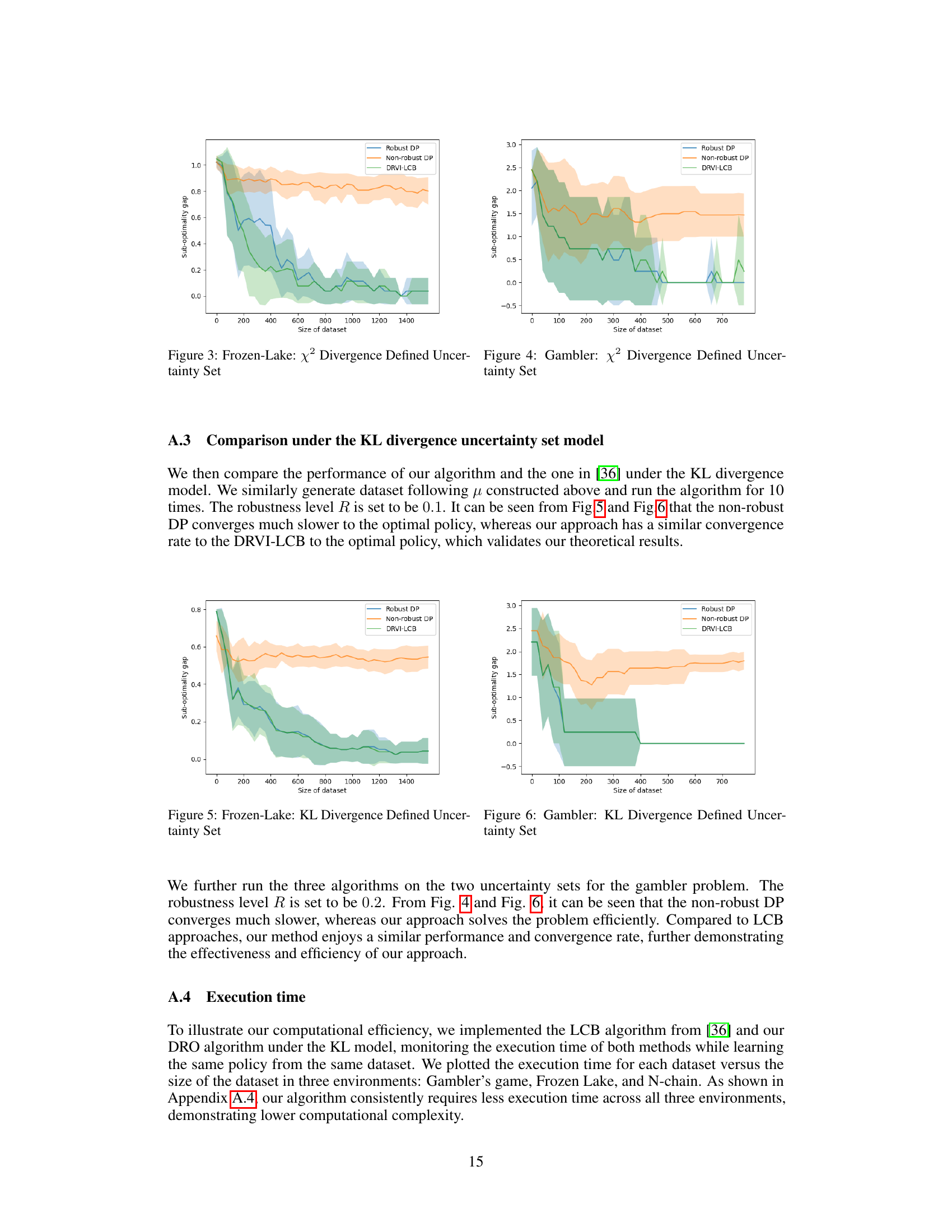
🔼 This figure compares three algorithms (Robust DP, Non-robust DP, and DRVI-LCB) under the total variation uncertainty set model on the Frozen Lake problem. The x-axis represents the size of the dataset, and the y-axis represents the sub-optimality gap. The shaded areas around the lines represent the standard deviations of the results over multiple runs (10 runs in this case). The figure shows that the value function-based construction of our algorithm (Robust DP) has a smaller sub-optimality gap and converges faster than the distribution-based construction and the DRVI-LCB, demonstrating that our algorithm is less conservative and more effective.
read the caption
Figure 1: Frozen-Lake: TV Distance Defined Uncertainty Set

🔼 This figure compares the performance of three algorithms (Robust DP, Non-robust DP, and DRVI-LCB) on the Frozen-Lake problem under the chi-squared divergence uncertainty model. The x-axis represents the size of the dataset used to train the algorithms. The y-axis represents the sub-optimality gap, a measure of how far the performance of each algorithm is from the optimal policy. The shaded areas around the lines represent the standard deviation of the results across multiple runs of each algorithm. The figure shows that the Robust DP algorithm converges faster and achieves a lower sub-optimality gap compared to the other two algorithms.
read the caption
Figure 3: Frozen-Lake: x² Divergence Defined Uncertainty Set

🔼 The figure shows the comparison of three algorithms under the total variation uncertainty set model for the FrozenLake problem. The x-axis represents the size of the dataset, while the y-axis represents the sub-optimality gap. The three algorithms are Robust Value Iteration (our algorithm using value function-based construction), Distribution-based Robust Value Iteration (our algorithm using distribution-based construction), and DRVI-LCB (baseline algorithm). The shaded area represents the standard deviation of 10 independent runs of each algorithm. The results demonstrate that our algorithm using the value function-based construction achieves better performance (smaller sub-optimality gap and faster convergence) compared to the baseline and the distribution-based construction.
read the caption
Figure 1: Frozen-Lake: TV Distance Defined Uncertainty Set
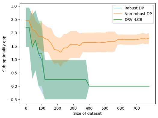
🔼 The figure compares the performance of three algorithms (Robust DP, Non-robust DP, and DRVI-LCB) on the Gambler problem under x² divergence uncertainty. The x-axis represents the size of the dataset used to train the algorithms, and the y-axis represents the sub-optimality gap, which measures how far the performance of the learned policy is from the optimal policy. The shaded area around each line shows the standard deviation across multiple runs. The results illustrate how our robust approach significantly outperforms the non-robust approach, demonstrating the benefits of using robustness measures, especially when working with limited data.
read the caption
Figure 4: Gambler: x² Divergence Defined Uncertainty Set

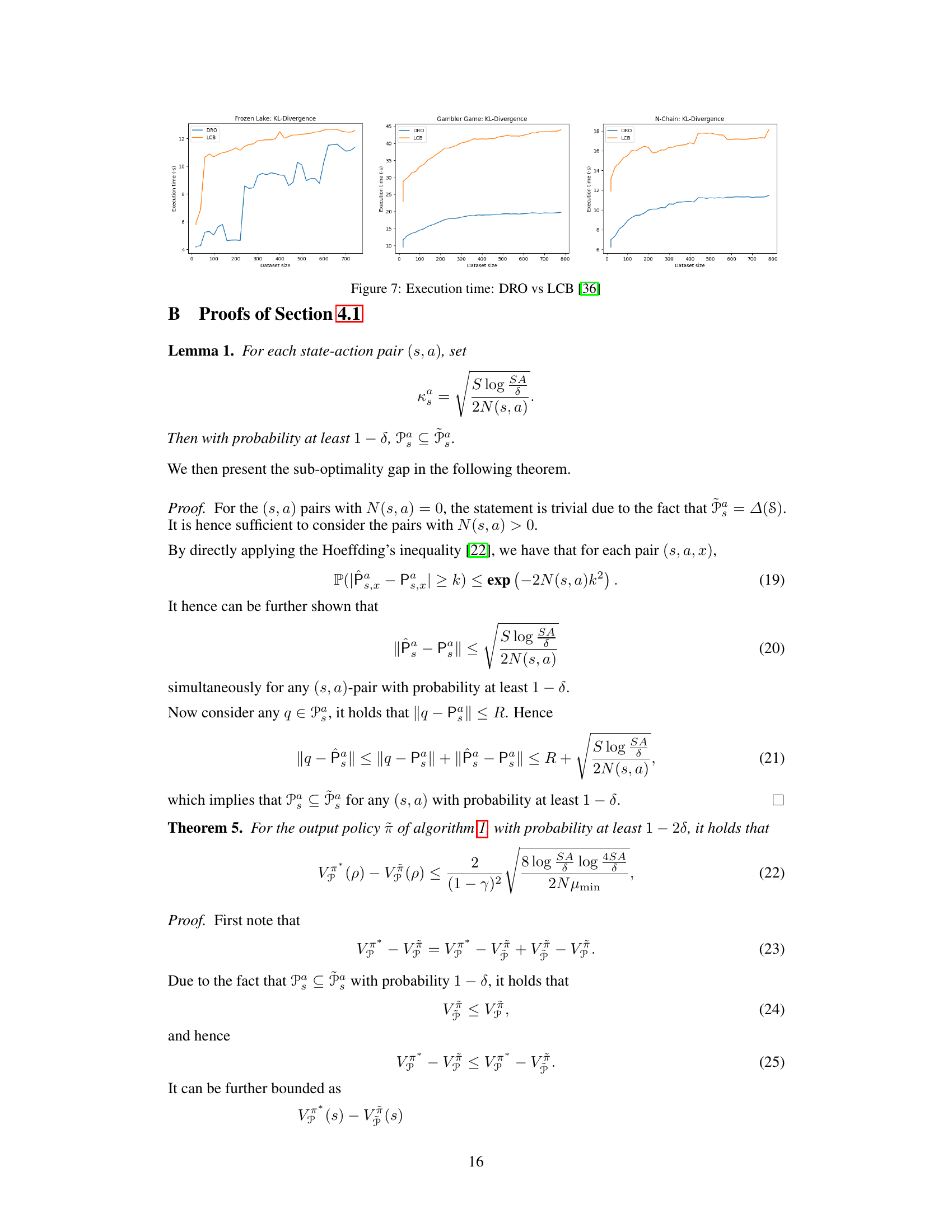
🔼 This figure compares the execution time of the proposed DRO algorithm and the LCB algorithm from [36] across three different environments: Frozen Lake, Gambler’s game, and N-Chain. The x-axis represents the dataset size, and the y-axis represents the execution time in seconds. The results show that, regardless of the environment, the DRO algorithm consistently demonstrates faster execution times, particularly as the dataset size increases, highlighting its improved computational efficiency.
read the caption
Figure 7: Execution time: DRO vs LCB [36]
Full paper#
