↗ OpenReview ↗ NeurIPS Homepage ↗ Chat
TL;DR#
Analyzing and optimizing convolutional neural networks (CNNs) is challenging due to the complexity of convolutions, especially when dealing with second-order optimization methods. Existing methods often suffer from high memory consumption and slow computation times, hindering their practical use in large-scale deep learning. Many hyper-parameters and additional features further complicate analysis and development.
This research presents a novel approach based on tensor networks (TNs) to represent convolutions. By viewing convolutions as TNs and leveraging the einsum library for efficient evaluation, the authors demonstrate significant speedups up to 4.5x for a recently proposed KFAC variant while substantially reducing memory usage. They derive concise formulas for various autodiff operations and curvature approximations and provide transformations that simplify computations, thus making the exploration of algorithmic ideas far easier. The TN implementation also enables a new hardware-efficient tensor dropout method.
Key Takeaways#
Why does it matter?#
This paper is crucial for researchers working with convolutional neural networks (CNNs) and second-order optimization methods. It offers significant speed and memory improvements for existing techniques, enabling more frequent updates and larger batch sizes. Additionally, the introduction of a novel tensor network perspective simplifies complex computations, opening up new avenues for algorithmic innovation and improving the efficiency of deep learning model development.
Visual Insights#
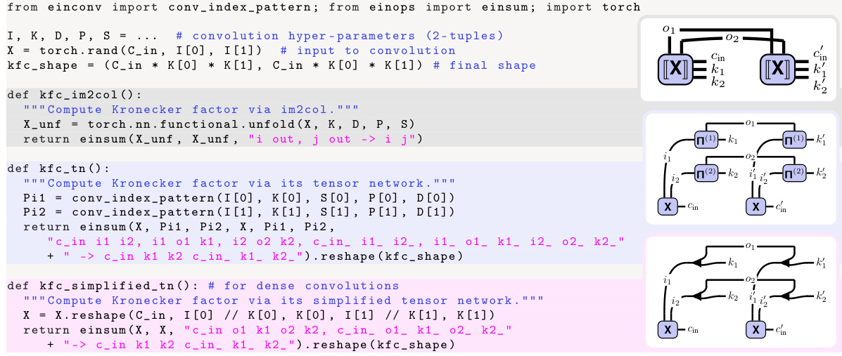
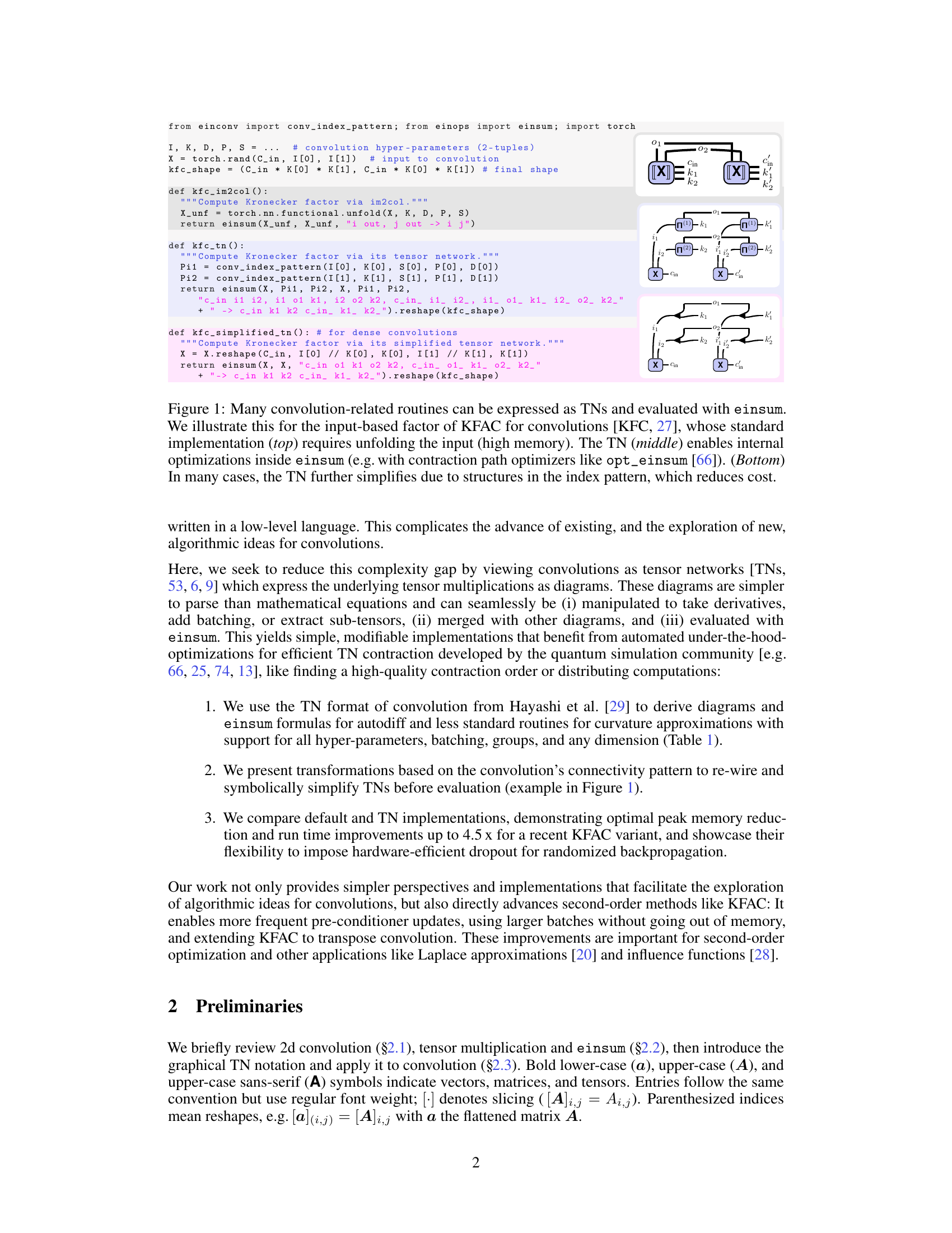
This figure demonstrates how various convolution-related operations can be represented as tensor networks (TNs) and efficiently computed using einsum. It focuses on the input-based Kronecker factor (KFC) for KFAC (Kronecker-factored approximate curvature), a second-order optimization method. The figure compares three approaches: a standard implementation using im2col (requiring unfolding and thus high memory), a TN representation which utilizes einsum for efficient tensor multiplications (and allows for internal optimization within einsum), and a further simplified TN leveraging structural properties of the index pattern for even greater efficiency. The figure highlights the simplicity and expressiveness of the TN approach for convolutions.

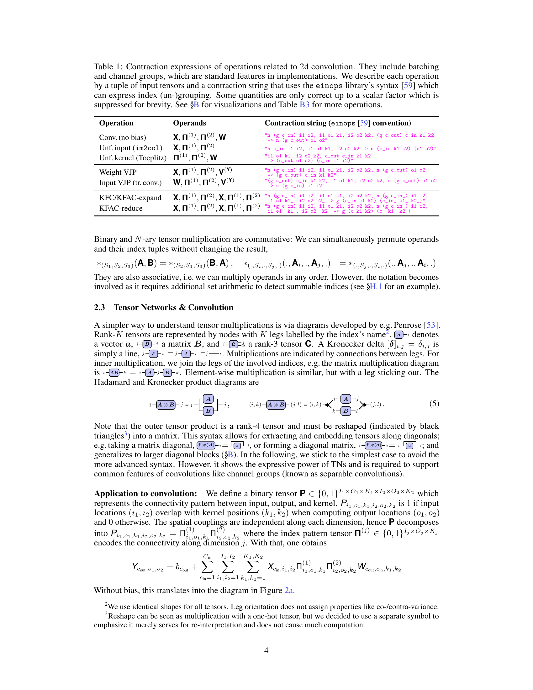
This table lists the einsum contraction strings for various operations related to 2D convolutions, including convolutions themselves, the unfolding of inputs and kernels, vector-Jacobian products (VJPs), and Kronecker-factored curvature approximations (KFC/KFAC). It shows how these operations can be expressed concisely and efficiently using the
einopslibrary’s syntax, incorporating batching and channel grouping. Note that some scalar factors are omitted for brevity.
In-depth insights#
Einsum Convolutions#
The concept of “Einsum Convolutions” suggests a novel approach to implementing convolutions using Einstein summation (einsum). This approach leverages the expressiveness of einsum to represent the tensor operations inherent in convolutions in a more compact and efficient manner. By viewing convolutions as tensor networks, the underlying tensor multiplications become visually clear through diagrams, simplifying analysis and manipulation. This framework facilitates the derivation of autodiff operations and the simplification of calculations for curvature approximations. Furthermore, it opens possibilities for hardware-efficient optimizations and novel algorithms not readily apparent with traditional methods. The core innovation lies in representing convolutions within the einsum framework, directly tackling memory-intensive operations like im2col and enabling streamlined computations for second-order methods. This offers significant advantages in memory efficiency and computational speed, especially for large-scale models.
TN Autodiff#
The concept of “TN Autodiff” suggests a novel approach to automatic differentiation (Autodiff) within the framework of tensor networks (TNs). This method leverages the visual and algebraic properties of TNs to represent and manipulate the computational graphs inherent in Autodiff. Key advantages likely include simplified derivative calculations, improved memory efficiency by avoiding explicit unfolding operations common in traditional convolutions, and enhanced expressiveness through intuitive diagrammatic manipulation. This approach offers a unique combination of symbolic and numerical computation, facilitating the exploration of complex Autodiff operations, such as higher-order derivatives, in a more accessible and potentially more efficient manner. The resulting implementations could offer significant performance improvements, especially for computationally demanding tasks like second-order optimization in deep learning models. However, challenges might arise from the complexity of optimizing TN contractions and the need for specialized software to efficiently evaluate the resulting einsum expressions. The potential for hardware acceleration and parallelization should be carefully considered in practical implementations. Overall, “TN Autodiff” presents a promising avenue for advancing Autodiff capabilities by harnessing the power of tensor networks, but thorough benchmarking and software development are crucial to fully realize its benefits.
KFAC Advances#
The paper explores Kronecker-factored approximate curvature (KFAC) methods, focusing on improving their efficiency for convolutional neural networks (CNNs). A key advancement is the use of tensor network (TN) representations to simplify convolutions and their associated computations. This TN approach allows for more efficient evaluation of KFAC’s components, particularly the input-based Kronecker factor, often a major computational bottleneck. Symbolic simplifications of the TNs are performed based on the structure of index patterns representing different convolutional types (dense, downsampled etc.), further optimizing calculations. This leads to significant speedups (up to 4.5x in experiments) and reduced memory overhead. The framework’s flexibility extends to handling various convolution hyperparameters and enabling KFAC for transpose convolutions, an area not well-addressed in existing libraries. The use of einsum is also a pivotal element in streamlining computations, leveraging its capabilities for efficient tensor contractions. Overall, the proposed enhancements demonstrate a compelling advancement in second-order optimization for CNNs, improving both speed and memory efficiency.
TN Simplifications#
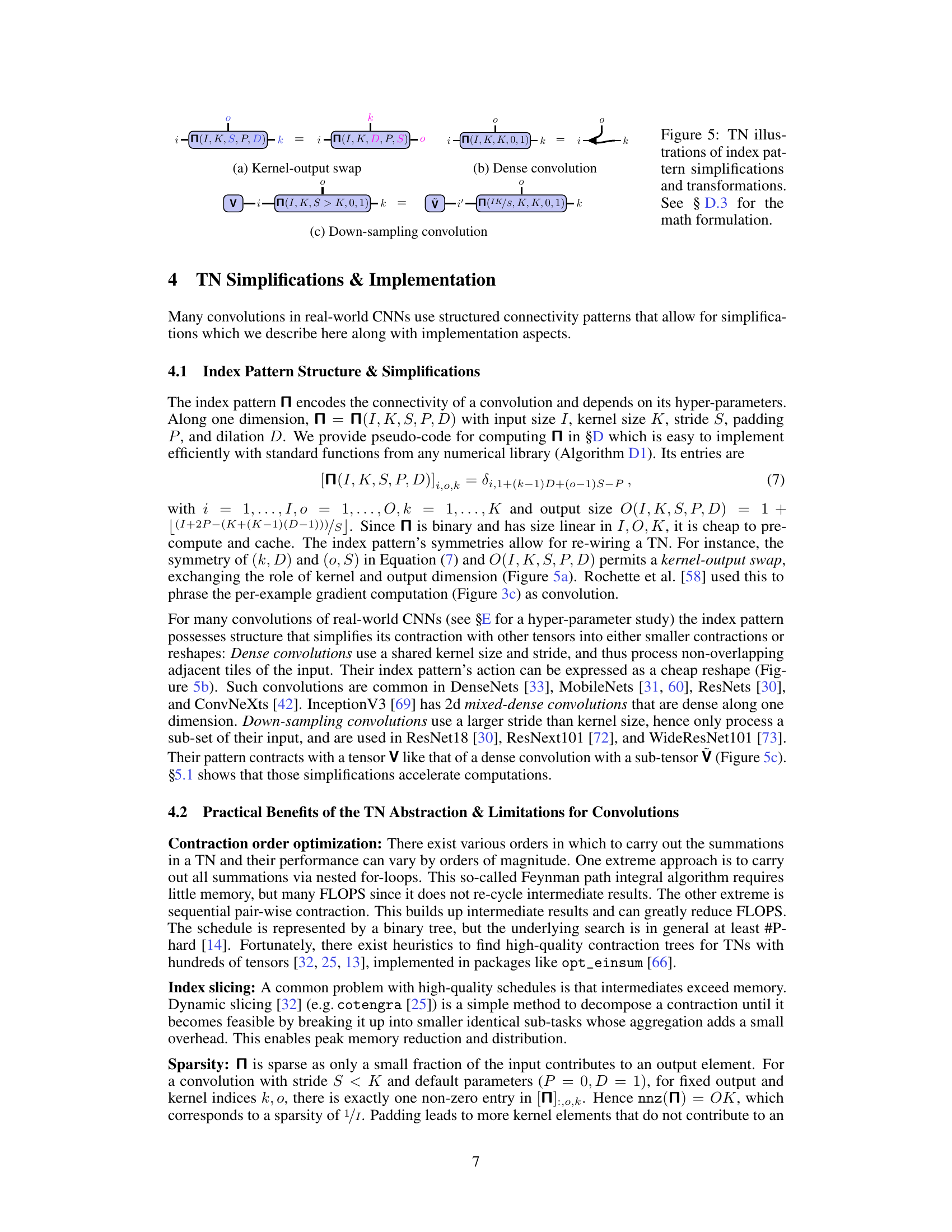
The heading ‘TN Simplifications’ likely refers to optimizations applied to tensor network (TN) representations of convolutions. The core idea is that many real-world convolutional neural networks utilize structured patterns in their connectivity. This section would detail how these structural regularities are leveraged to simplify TN calculations. Specific techniques might include exploiting symmetries in index patterns, identifying and exploiting dense or downsampling convolution patterns (reducing computation through reshaping), or clever re-wiring of TN diagrams to minimize computational costs. The authors likely demonstrate that these simplifications significantly reduce computational complexity and memory requirements, leading to faster and more efficient implementations of convolution operations within the TN framework. Hardware-specific considerations may also be incorporated to optimize the simplified TNs for specific architectures.
Runtime Boost#
The concept of “Runtime Boost” in the context of optimizing convolutional neural networks (CNNs) using tensor network (TN) representations is intriguing. The core idea revolves around expressing CNN operations, including complex ones like second-order methods, as TNs, enabling efficient evaluation via einsum. Significant speed-ups are reported, potentially reaching 4.5x in specific cases. This improvement stems from several factors: (1) Einsum’s inherent optimization capabilities for tensor contractions; (2) TN structure revealing hidden symmetries in CNN operations, which leads to streamlined computations; (3) Exploiting structured connectivity patterns in many common CNNs (e.g., dense or down-sampling convolutions) resulting in further simplifications. However, it is important to note that runtime gains might not always be substantial, especially for less common operations and implementations lacking significant optimization opportunities. Hardware-specific optimizations may play a crucial role in achieving these speed-ups. The paper’s comprehensive analysis includes various experiments across diverse architectures and tasks, highlighting when TN methods provide the most significant advantage in reducing computational costs. Memory efficiency and flexibility in handling hyperparameters also seem to be strong points of this approach.
More visual insights#
More on figures

This figure illustrates the tensor network (TN) representation of a 2D convolution and how it relates to the matrix multiplication view. Panel (a) shows the TN diagram for convolution, clearly depicting the connections between the input tensor (X), kernel (W), and output (Y). The index pattern tensors, Π(1) and Π(2), explicitly represent the connectivity along each spatial dimension. Panels (b) and (c) demonstrate how input unfolding (im2col) and kernel unfolding can be viewed as specific TN structures derived from the main convolution TN in (a). This highlights the paper’s core idea of representing convolutions as TNs for easier analysis and manipulation.

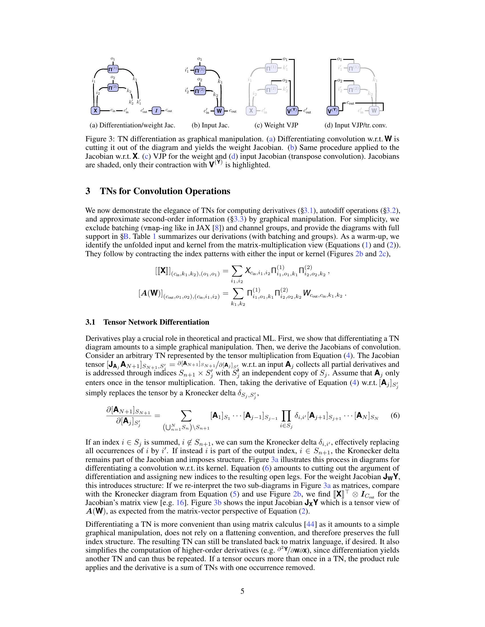
This figure demonstrates the process of TN differentiation as a graphical manipulation. It shows how differentiating a tensor network (TN) diagram for convolution w.r.t weights (W) or inputs (X) results in simpler diagrams. Panel (a) shows differentiating w.r.t W (weight Jacobian), and (b) shows the differentiation w.r.t X (input Jacobian). Panels (c) and (d) depict the vector-Jacobian products (VJPs) for weight and input, respectively, highlighting the connection to transpose convolutions. Shaded areas represent Jacobians, and only their contractions with V(Y) are highlighted.

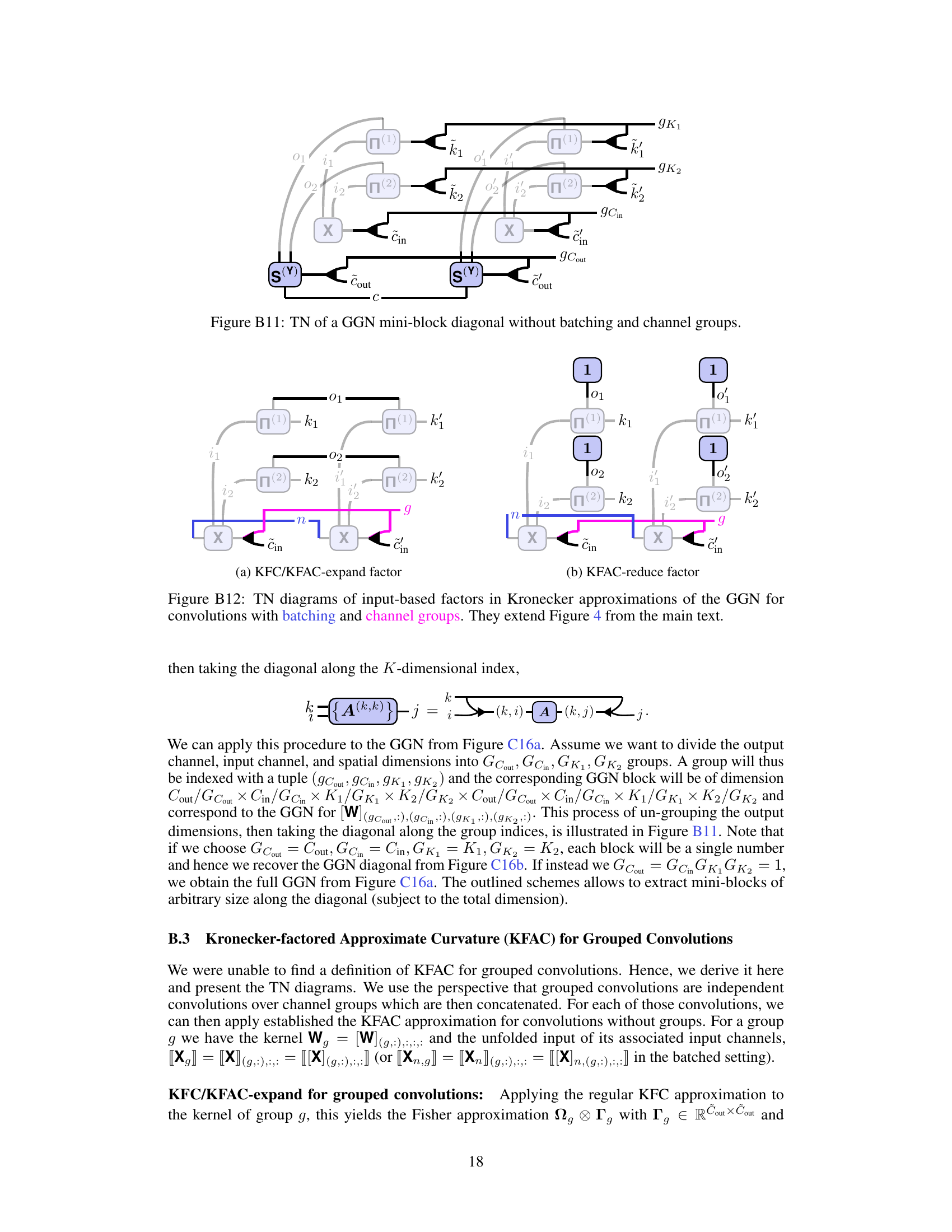
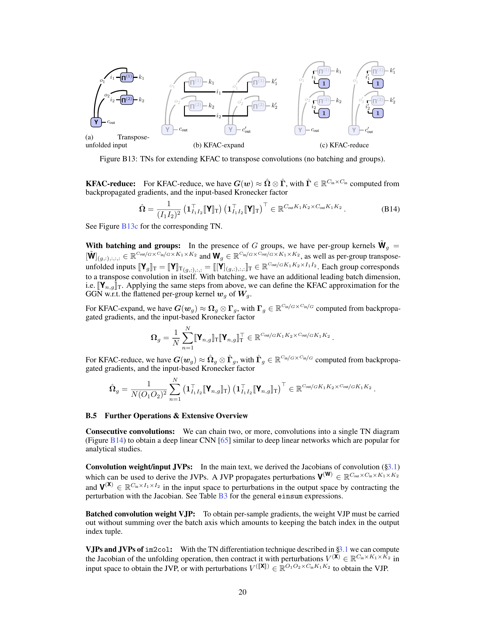
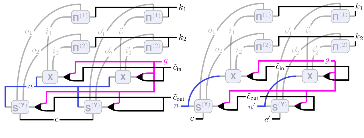
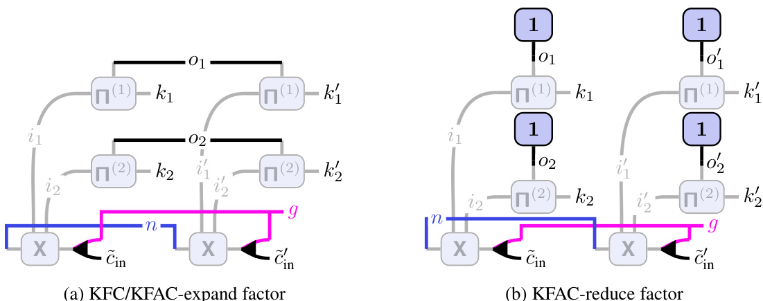
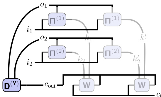
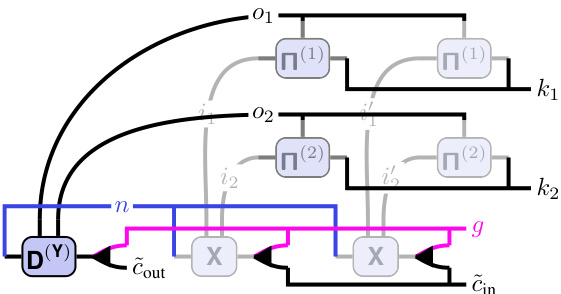
This figure shows the tensor network (TN) diagrams for the input-based Kronecker factors in two popular Kronecker-factored approximate curvature methods: KFAC-expand and KFAC-reduce. The diagrams illustrate how these factors are computed using tensor network operations. The unfolded input is represented by a shaded area, emphasizing its role in the calculations. The diagrams highlight the differences in connectivity patterns between the KFAC-expand and KFAC-reduce approaches, reflecting variations in how they approximate the Fisher/Generalized Gauss-Newton (GGN) matrix.

This figure illustrates how tensor networks (TNs) can simplify the computation of convolution-related routines, particularly the input-based factor of Kronecker-factored approximate curvature (KFAC). The figure compares three approaches: a standard implementation using unfolding (im2col), a TN implementation using einsum, and a simplified TN implementation leveraging index pattern structures. The TN approach avoids memory-intensive unfolding, allows for internal optimizations within einsum, and can lead to further simplifications based on the structure of the index pattern, resulting in significant computational cost reduction.
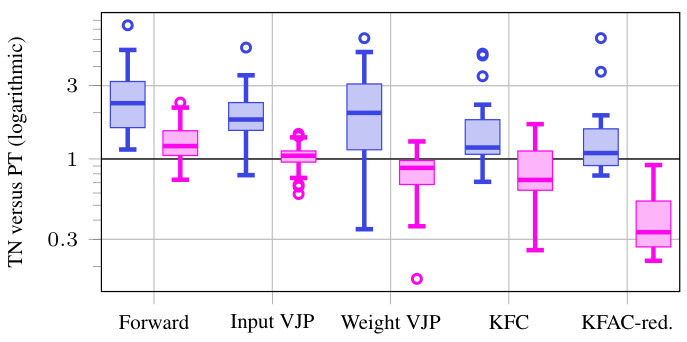
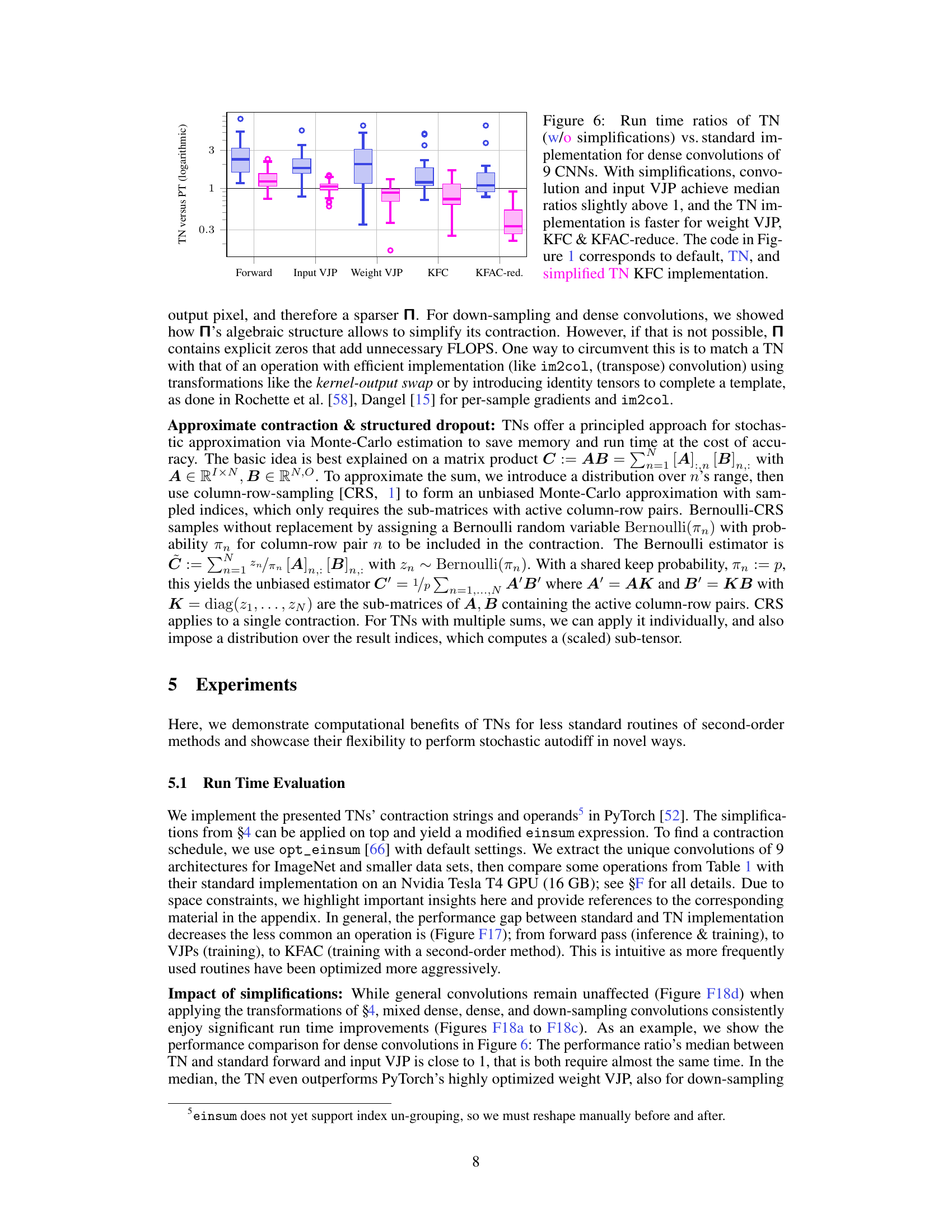
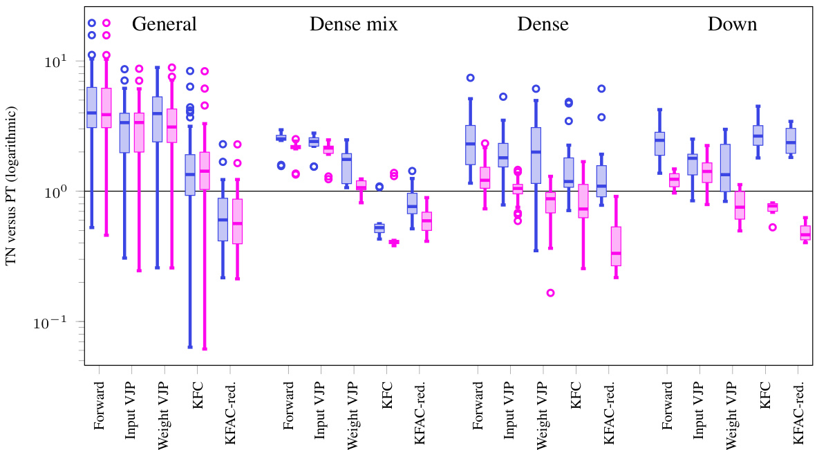
This figure compares the performance (run time) of tensor network (TN) implementations of various convolution-related operations with their standard PyTorch counterparts. It shows that TNs, even without simplifications, are comparable in speed for forward and input VJP, but significantly outperform standard PyTorch for weight VJP, KFC and KFAC-reduce, especially after simplifications are applied. The comparison uses dense convolutions from nine different Convolutional Neural Networks (CNNs).

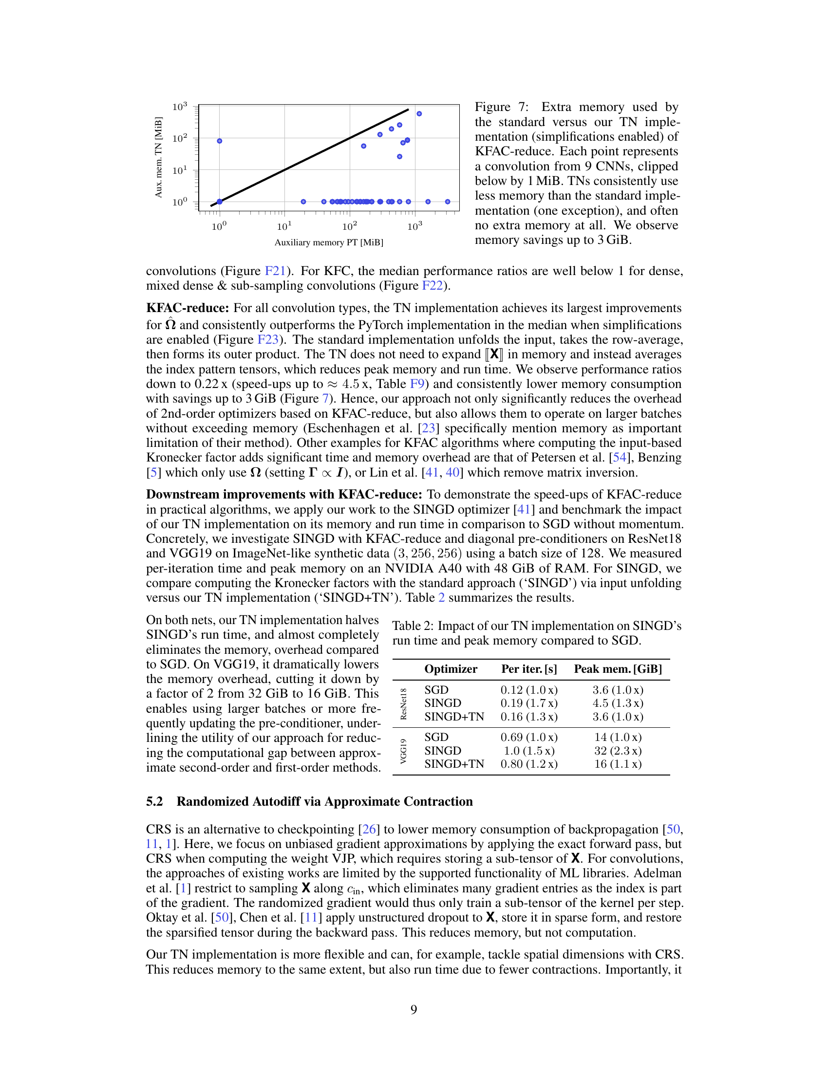
This figure compares the auxiliary memory usage of the standard implementation versus the tensor network (TN) implementation of the KFAC-reduce algorithm for various convolutional layers in nine different Convolutional Neural Networks (CNNs). The y-axis represents the auxiliary memory used by the TN implementation, while the x-axis represents the auxiliary memory used by the standard implementation. Each point corresponds to a specific convolutional layer in one of the nine CNNs, and the values are clipped at a minimum of 1 MiB. A line of best fit is included to emphasize the trend of reduced memory usage for the TN implementation. The results indicate that the TN implementation consistently uses less memory than the standard implementation, with some cases showing a reduction of up to 3 GiB.

The figure shows that sampling spatial axes is more effective than channels in reducing approximation error when using Bernoulli-CRS for stochastic gradient approximation. This is demonstrated on both real-world and synthetic data using the untrained All-CNN-C model for CIFAR-100. The results show that for the same memory reduction, spatial sampling achieves lower error compared to channel sampling. This suggests a more efficient strategy for reducing computational cost in stochastic gradient approximation.
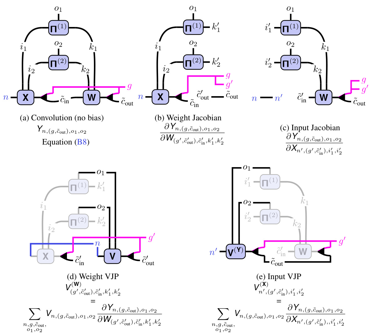
This figure demonstrates how taking derivatives of a tensor network (TN) representation of a convolution can be done via simple graphical manipulations. It shows four diagrams, each representing a different operation: (a) Differentiating with respect to the kernel (W) results in a cut to the network that isolates the Jacobian of the convolution with respect to the kernel. (b) Differentiating with respect to the input (X) similarly results in a cut showing the Jacobian with respect to the input. (c) The vector-Jacobian product (VJP) for the weights illustrates how the gradient flows back through the network. (d) The VJP for the input shows the equivalent for the input, which is the transpose convolution (also demonstrating that the transpose convolution is cleanly described as the corresponding VJP). The shaded areas highlight the Jacobians, and the connection to the V(Y) vector emphasizes how the contraction produces the final result.
This figure illustrates how the tensor network (TN) representation of a convolution simplifies the process of computing derivatives. It shows that differentiating a convolution with respect to its weights (W) or inputs (X) involves a simple graphical manipulation: cutting the corresponding tensor out of the TN diagram. The resulting diagrams visually represent the weight Jacobian (∂Y/∂W), input Jacobian (∂Y/∂X), weight vector-Jacobian product (VJP for W), and input VJP (which is equivalent to a transpose convolution). Shaded areas highlight the Jacobian tensors, showing how they contract with the vector V(Y) during backpropagation.

This figure demonstrates how tensor network (TN) diagrams can be used to visualize and simplify the process of differentiating convolutions. It shows how taking the derivative with respect to weights (W) or inputs (X) can be represented graphically as cutting those parts from the TN diagrams. The resulting diagrams represent the Jacobians (weight Jacobian, input Jacobian), which capture the sensitivity of the output to changes in weights and inputs. The figure also illustrates the computation of vector-Jacobian products (VJPs), a crucial step in backpropagation, by showing how they can be obtained by contracting the Jacobians with the gradient of the loss function (V(Y)).
This figure demonstrates how convolution-related operations can be represented and computed using tensor networks (TNs) and the einsum function. It uses the example of the Kronecker-factored curvature (KFC) for convolutions, comparing three different approaches: a standard implementation (requiring memory-intensive unfolding of the input), a TN representation (allowing for internal optimizations within einsum), and a simplified TN representation (further reducing computational cost due to exploiting structural patterns in the index pattern).

This figure illustrates the tensor network (TN) representations of a 2D convolution and how it relates to matrix multiplication. Panel (a) shows the TN representation of the convolution, highlighting the connections between input, output, and kernel tensors through index pattern tensors. Panels (b) and (c) illustrate how the input and kernel tensors can be unfolded and reshaped to allow for matrix multiplication. The figure emphasizes the use of index pattern tensors (Π) to explicitly define the connectivity within each dimension, making the TN representation a powerful tool for analysis and manipulation of convolutions.

This figure illustrates the tensor network (TN) representation of a 2D convolution. Panel (a) shows the TN diagram of a 2D convolution, highlighting the connections between the input tensor (X), the kernel (W), and the output tensor (Y). The connections are explicitly represented by index pattern tensors Π(1) and Π(2), which encode the spatial relationships between the input, kernel, and output along the respective dimensions (I1, I2, O1, O2, K1, K2). Panel (b) shows how the input is unfolded (im2col) to form a matrix, explicitly illustrating the connectivity. Panel (c) shows an analogous unfolding for the kernel, again emphasizing the connectivity in the matrix multiplication. This depiction helps bridge the intuitive understanding of a convolution’s sliding window approach with a more formal tensor network analysis.
This figure illustrates how to perform differentiation in a tensor network. It shows that differentiating a tensor network diagram is equivalent to a simple graphical manipulation. The diagrams (a) through (d) illustrate how to compute weight Jacobian, input Jacobian, and Jacobian-vector products (VJPs) graphically by removing parts of the diagram. Shaded areas represent the Jacobians, and their contraction with V(Y) is highlighted.

This figure illustrates the tensor network (TN) diagrams for various operations related to 2D convolutions, including the forward pass, Jacobians (weight and input), and vector-Jacobian products (VJPs, weight and input). The diagrams incorporate batching and channel groups, adding complexity compared to the simpler diagrams in Figures 2 and 3. Shading is used in the VJP diagrams to highlight the Jacobian tensors. The figure extends the concepts presented in the main text to more realistic scenarios by incorporating these additional factors.

This figure demonstrates how to compute the derivatives of a convolutional layer using tensor network diagrams. Panel (a) shows how differentiating with respect to the weights (W) is represented graphically; cutting the weight tensor from the network yields the weight Jacobian. Panel (b) shows the same process for differentiating with respect to the input (X), resulting in the input Jacobian. Panels (c) and (d) illustrate the vector-Jacobian product (VJP) for weights and the input Jacobian (related to transpose convolution), respectively. The Jacobians are highlighted in gray, and their contractions with V(Y) are emphasized.
This figure demonstrates how tensor network (TN) diagrams simplify the process of differentiation in convolutions. Each sub-figure (a-d) shows a TN representation of a different autodiff operation: (a) differentiating the convolution with respect to the kernel (weight Jacobian), (b) differentiating with respect to the input (input Jacobian), (c) calculating the vector-Jacobian product (VJP) for the weights, and (d) calculating the VJP for the input (transpose convolution). The shaded areas represent the Jacobian tensors, and their contractions with the vector V(Y) are highlighted.

This figure illustrates how to represent and compute Kronecker factors for convolutions using Tensor Networks (TNs). The standard method (top) uses im2col, which requires unfolding the input tensor, leading to high memory usage. The TN representation (middle) allows for internal optimizations within the einsum function (especially using contraction path optimizers like opt_einsum), improving efficiency. The bottom part shows that, in many situations, the TN can be simplified even further due to the specific structure of the index patterns of convolutions, again resulting in memory and computational savings.
This figure illustrates how tensor networks (TNs) and einsum can simplify the computation of convolution-related routines. The example shown is the input-based factor of Kronecker-factored curvature (KFC) for convolutions. The standard implementation is memory-intensive because it requires unfolding the input. The TN representation allows for internal optimizations within the einsum function, such as contraction path optimization. Finally, the TN representation can be further simplified based on structural properties of the index patterns, leading to additional computational savings.

This figure demonstrates how Kronecker-factored curvature (KFC) approximation for convolutions can be represented as tensor networks (TNs) and efficiently evaluated using einsum. It compares three approaches: a standard implementation using im2col (requiring input unfolding and thus high memory), a TN representation which allows for einsum’s internal optimizations, and a simplified TN representation that leverages index pattern structures to reduce computational cost. The figure visually illustrates these methods with diagrams and highlights the memory and computational advantages of using TNs.

This figure presents a comparison of the runtime performance between a Tensor Network (TN) implementation and a standard PyTorch implementation for various convolution operations. The results are shown for nine different Convolutional Neural Networks (CNNs), focusing on dense convolutions. The x-axis represents different operations (Forward, Input VJP, Weight VJP, KFC, KFAC-reduce), and the y-axis shows the ratio of TN runtime to the standard PyTorch runtime. The figure illustrates that without simplifications, the TN implementation is generally slower than PyTorch’s implementation; however, when simplifications are applied, the TN’s performance improves significantly, becoming comparable or even faster than PyTorch’s in several cases.

This figure compares the performance of the Tensor Network (TN) implementation of convolutions against the standard PyTorch implementation for dense convolutions across 9 different Convolutional Neural Networks (CNNs). It shows run-time ratios, indicating how much faster or slower the TN method is compared to the standard method. Two sets of results are presented: one without any simplifications applied to the TN approach and another with simplifications enabled. The results show that with simplifications, the TN method is either comparable to, or faster than, the standard PyTorch implementation for most operations, highlighting the efficiency gains achieved.

This figure compares the performance of the Tensor Network (TN) implementation of dense convolutions against the standard PyTorch implementation. It shows run time ratios for various operations including forward pass, input VJP, weight VJP, KFC, and KFAC-reduce. The results indicate that with simplifications, the TN implementation is competitive with or even outperforms PyTorch for some operations, highlighting the efficiency of the TN approach, especially for more complex computations like weight VJP, KFC, and KFAC-reduce.
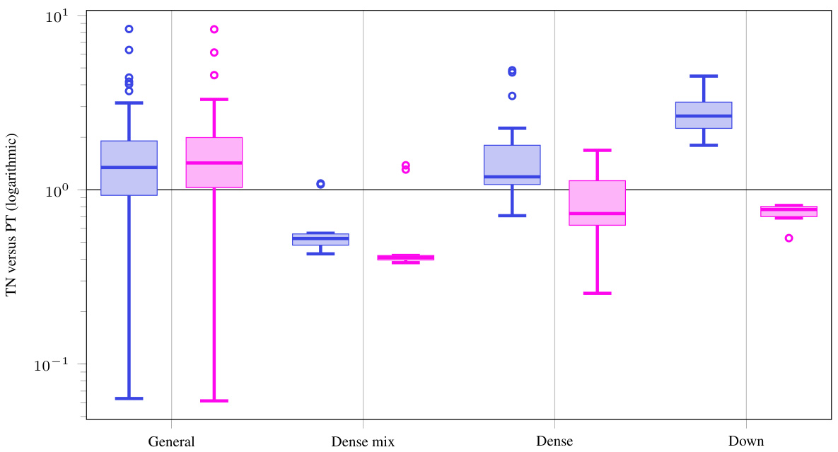
This figure presents the performance comparison of the Tensor Network (TN) approach with the standard implementation for computing the Kronecker factors in KFAC (KFC and KFAC-reduce). It shows the run-time ratios for various operations in dense convolutions across 9 different Convolutional Neural Networks (CNNs). Two sets of results are shown: those without TN simplifications (blue boxes) and those with simplifications (magenta boxes). The results indicate that TN implementations with simplifications are comparable or faster than the standard approach for most operations, demonstrating efficiency gains for weight VJP and the approximation of KFAC.
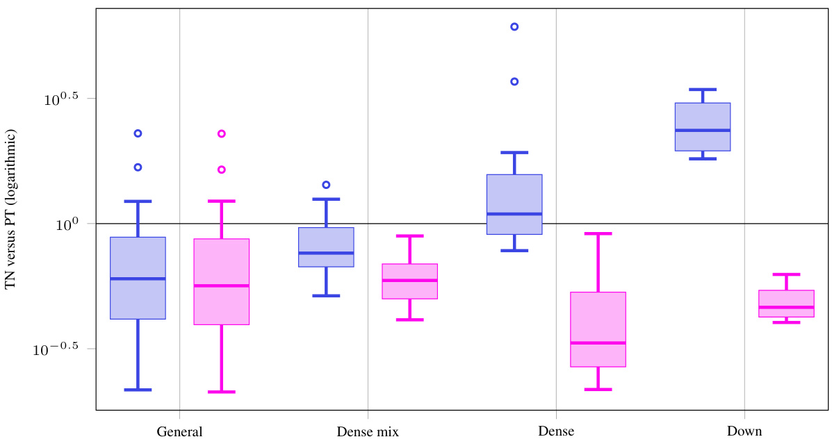
This figure shows the performance comparison between the standard PyTorch implementation and the proposed Tensor Network (TN) implementation for dense convolutions across 9 different Convolutional Neural Networks (CNNs). The results are presented as the ratio of TN run time to PyTorch run time, with lower ratios indicating that TN is faster. Two sets of box plots are shown, one for the TN implementation without simplifications (showing that TN is often slower without optimizations) and one for the TN implementation with the simplifications described in the paper. The simplifications lead to improved performance, particularly for weight VJP, KFC and KFAC-reduce. The figure also highlights the equivalence between three different implementations of the KFC (Kronecker-factored curvature) routine (default, TN, and simplified TN) to show how the TN approach is superior.
More on tables
This table lists the einsum contraction strings for various operations related to 2D convolutions, including convolutions themselves, their Jacobians, VJPs, and curvature approximations like KFAC. It shows the input tensors and the corresponding einsum string for each operation, enabling concise representation of these computations. The table also notes that some scalar factors are omitted for brevity and references supplementary material for visualizations and a more comprehensive list of operations.

This table shows the einsum contraction strings for various operations related to 2D convolutions, including convolutions themselves, their Jacobian, vector-Jacobian products (VJPs), and Kronecker-factored curvature approximations like KFAC. It encompasses batching and channel groups and aims to provide concise formulas using the
einopslibrary’s syntax. The table also references a more detailed explanation and visualization in the supplement.

This table presents the einsum contraction expressions for various operations related to 2D convolutions, including standard operations like convolution itself and its Jacobian, and second-order methods such as KFAC. It shows the input tensors required and the einsum contraction string using the einops library’s notation. Batching and channel groups are included, and the table notes that some scalar factors are omitted for brevity. Further visualizations and additional operations are available in the supplementary material.

This table lists the einsum contraction strings for various operations related to 2D convolutions, including convolutions themselves, their Jacobians, and popular curvature approximations like KFAC. It shows how to express these operations using the
einopslibrary’s syntax, which is compact and allows for flexible index manipulation. The table also includes batching and channel groups, common features in modern deep learning implementations. Note that some quantities are only accurate up to a scalar factor, which is omitted for brevity.

This table extends Table 1 from the main paper by providing a more extensive list of convolution and related operations. It includes operations such as convolution, unfolded input, unfolded kernel, folded output, transpose-unfolded input, weight VJP, input VJP, KFC/KFAC-expand, KFAC-reduce, GGN Gram matrix, GGN/Fisher diagonal, and approximate Hessian diagonals. For each operation, it specifies the operands and the contraction string using the einops library’s convention. The table shows that the operations include batching and channel groups, and are generalized to any number of spatial dimensions.

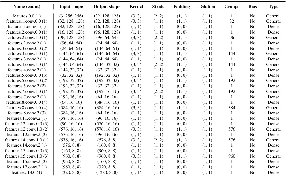
This table lists the hyperparameters of convolutional layers from nine different Convolutional Neural Networks. The networks are categorized by their dataset (CIFAR-10, CIFAR-100, Fashion MNIST, and ImageNet) and architecture (3c3d, 2c2d, All-CNN-C, AlexNet, ResNet18, ResNext101, ConvNeXt-base, InceptionV3, and MobileNetV2). For each convolutional layer, the table shows its name, input shape, output shape, kernel size, stride, padding, dilation, number of groups, whether a bias term is used, and the type of convolution (general, dense, down-sampling). The ‘count’ column indicates how many layers share the same hyperparameters.

This table presents the einsum contraction expressions for various operations related to 2D convolutions. It includes common operations such as convolution itself (with and without bias), unfolding of inputs and kernels, and the vector-Jacobian products (VJPs) for weights and inputs (relevant for backpropagation and transpose convolutions). It also covers Kronecker-factored curvature approximations such as KFC/KFAC expand and reduce. The table indicates the input tensors needed for each operation and provides the einsum contraction string using the einops library’s syntax, allowing for batching and channel grouping. Note that some quantities might be only correct up to a scalar factor, which is omitted for simplicity. For further details and visualizations, readers are referred to section B and Table B3 in the supplementary material.

This table extends Table 1 from the main paper by including more operations related to convolutions. It shows the operations’ operands, contraction strings (using the einops convention), and includes support for batching and channel groups, extending the coverage to various common operations beyond those presented in the main paper.

This table lists the einsum contraction strings for various operations related to 2D convolutions, including convolutions themselves, their Jacobians, vector-Jacobian products, and Kronecker-factored curvature approximations (KFC/KFAC). It includes support for batching and channel groups, and shows how to express these operations using the einops library’s syntax. Note that some quantities are approximate (up to a scalar factor). More details and visualizations can be found in Appendix B.

This table extends Table 1 from the main text by including more operations related to convolutions. It provides a comprehensive list of contraction expressions for various operations, including convolutions, Jacobian-vector products (JVPs), vector-Jacobian products (VJPs), Kronecker-factored approximate curvature (KFAC) variants, and Hessian approximations. Each operation is described by its operands and a contraction string using the einops library’s syntax. The table explicitly incorporates batching and channel groups, and indicates how the operations can be extended to higher dimensions.
This table extends Table 1 from the main paper by including more convolution-related operations and including batching and channel groups. The table includes the operands needed and einsum contraction strings for each operation. This is a comprehensive listing of many operations related to 2D convolutions.

This table presents a detailed breakdown of the forward pass performance for various convolutional neural networks (CNNs) across different categories (General, Dense mix, Dense, Down). For each CNN and layer, the table provides the run times for the Tensor Network (TN) implementation, the PyTorch (PT) implementation, and the performance factors (TN/PT and TN+opt/PT). The performance factors indicate the speedup or slowdown achieved by the TN implementation compared to the PT implementation. Lower values indicate better performance. The table provides detailed numbers for comparison. The CNNs are categorized into four groups: 3c3d (CIFAR-10), F-MNIST 2c2d, CIFAR-100 All-CNN-C, AlexNet, ResNet18, ResNext101, and ConvNeXt-base.

This table presents a detailed comparison of the forward pass performance between the Tensor Network (TN) implementation and the PyTorch (PT) implementation for various CNN architectures and convolution types. The table includes the run times for TN, TN with optimizations (TN+opt), and PT. For each architecture and convolution layer, the factor of TN/PT and TN+opt/PT, calculated using the run times, is given. This allows to compare the performance of the TN implementation against PyTorch’s highly optimized functions for the forward pass. The table is divided into sections for different datasets (CIFAR-10, Fashion MNIST, ImageNet), and each section shows results for different CNN architectures (3c3d, 2c2d, All-CNN-C, AlexNet, ResNet18, ResNext101, ConvNeXt-base) and their respective convolution layers.

This table presents a detailed breakdown of the forward pass performance comparison between the Tensor Network (TN) implementation and the PyTorch (PT) implementation for various CNNs. It provides the runtimes (in seconds) for both TN and PT, along with the performance factor (TN time / PT time). The performance factor indicates the speedup or slowdown of the TN implementation relative to the PT implementation. The table includes results for different convolution types (general, mixed-dense, dense, and down-sampling) and architectures to comprehensively assess the efficiency gains provided by the TN approach.

This table presents a detailed breakdown of the forward pass performance comparison between the proposed Tensor Network (TN) implementation and the standard PyTorch (PT) implementation across various CNN architectures and convolution types. For each CNN and convolution layer, the table reports the run times for the TN, TN with optimizations (TN+opt), and PT implementations, along with the corresponding performance factors (TN/PT and TN+opt/PT). The performance factor indicates the speed-up or slow-down achieved by the TN implementation relative to the PT implementation. A performance factor greater than 1 means the TN implementation is slower, while a factor less than 1 indicates the TN implementation is faster.

This table shows the einsum contraction strings for various operations related to 2D convolutions, including convolutions themselves, their Jacobians, and related quantities such as the Kronecker factors used in KFAC approximations. The table includes support for batching and channel groups and uses the einops library’s syntax for concise representation. Note that some scalar factors are omitted for brevity.

This table presents a detailed comparison of the forward pass performance between the Tensor Network (TN) implementation and the PyTorch (PT) implementation for various convolution types across different CNN architectures. It includes the run times for both TN and TN+opt (TN with simplifications), along with the corresponding PyTorch run times and performance factors (ratios of TN/PT and TN+opt/PT run times). The results are broken down by convolution type (General, Mixed dense, Dense, Down).

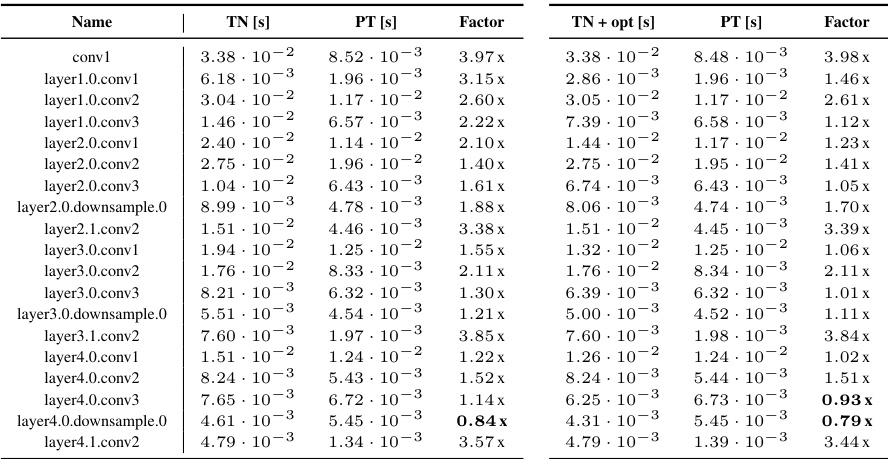
This table presents a detailed comparison of the performance of the KFAC-reduce factor computation using different methods (TN, TN+opt, and PT) across various CNN architectures and convolution types. For each convolution layer, the table provides the execution time in seconds for each method (‘TN [s]’, ‘PT [s]’, ‘TN + opt [s]’) and calculates the performance ratio (‘Factor’) which is the ratio of execution times between the TN-based methods and the PyTorch method (PT). Lower values for the ratio indicate that the TN-based method outperformed PyTorch.
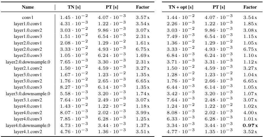
This table presents a detailed comparison of the run times for computing the input-based KFAC-reduce factor using different methods (TN, TN+opt, and PyTorch’s implementation) across various CNN architectures and convolution types. It provides the run times for each method (in seconds), and the performance ratios which represent the speed-up achieved by TN and TN+opt relative to PyTorch’s approach. The table helps demonstrate the efficiency gains obtained using the proposed Tensor Network (TN) methods, particularly when the simplifications in section 4 of the paper are applied.

This table lists contraction expressions (using einops syntax) for various operations related to 2D convolutions. It shows the input tensors required and the corresponding einsum-style contraction string. The operations covered include basic convolution (with and without bias), unfolding the input and kernel, vector-Jacobian products (VJPs), and components of Kronecker-factored curvature approximations (KFAC). Batching and channel groups are supported. Note that some scalar factors are omitted for brevity.
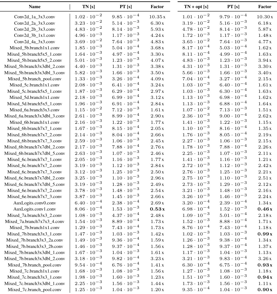
This table extends Table 1 from the main paper by including more operations related to 2D convolutions. It shows the operands and einsum contraction strings for various operations, including convolutions with and without bias, unfolded input and kernel, VJPs (vector-Jacobian products), JVPs (Jacobian-vector products), KFAC (Kronecker-factored approximate curvature) expansions and reductions, and approximations for the Hessian diagonal. The table also includes support for batching and channel groups, and indicates how to generalize to higher dimensions.
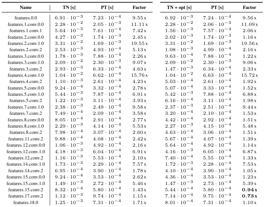
This table extends Table 1 from the main paper by including batching and channel groups, providing more comprehensive contraction expressions for various operations related to 2D convolutions. It covers a wider range of operations, including convolutions, Jacobian-vector products, and various curvature approximations. The table is organized by operation, providing the operands and contraction strings for each using einops library syntax.

This table provides detailed results for forward pass performance comparison on GPU. It includes the runtimes and performance factors (ratio of TN implementation to PT) for different convolution types across various CNN architectures (3c3d, F-MNIST 2c2d, CIFAR-100 All-CNN-C, AlexNet, ResNet18, ResNext101, and ConvNeXt-base). For each architecture and convolution, the table shows the runtime for both the standard TN implementation and TN + opt (with simplifications), alongside the corresponding PyTorch (PT) runtime and the performance factor. This allows for a detailed comparison of performance improvements achieved with the proposed tensor network (TN) approach.

This table presents a detailed breakdown of the forward pass performance comparison between the Tensor Network (TN) and PyTorch (PT) implementations across various CNN architectures on a GPU. The table is organized by architecture (3c3d, F-MNIST 2c2d, CIFAR-100 All-CNN-C, AlexNet, ResNet18, ResNext101, ConvNeXt-base, Inception V3, MobileNetV2), then by layer name within each architecture. For each layer, the table provides the run time in seconds for the TN implementation, the PT implementation, and the TN implementation with optimizations applied (TN+opt). Finally, it shows the performance ratio, which is the TN run time divided by the PT run time. A ratio less than 1 indicates that the TN implementation is faster than PT. The table helps demonstrate the relative speed improvements of the TN-based approach across different network types and layers.

This table lists the einsum contraction strings for various operations related to 2D convolutions, including convolutions themselves, their Jacobians (input and weight), and second-order methods like Kronecker-factored approximate curvature (KFAC). It shows the input tensors required for each operation and the corresponding einsum string using the einops library’s convention. Note that some quantities are only correct up to a scalar factor, which is omitted for brevity. Further details, including visualizations, are available in Section B and Table B3.

This table presents a detailed breakdown of the forward pass performance comparison between the Tensor Network (TN) implementation, the simplified TN+opt implementation, and PyTorch’s default implementation (PT) for various convolution types across several architectures. The table displays the runtimes (in seconds) for each implementation and calculates the performance factor by dividing the runtime of the TN implementations by the PT runtime. A performance factor less than 1 indicates the TN-based method is faster. The results are categorized by architecture and convolution type, providing a comprehensive assessment of the efficiency gains achieved with the proposed tensor network approach.

This table presents a detailed comparison of the forward pass performance between the Tensor Network (TN) implementation and the PyTorch implementation (PT) for various convolutional layers across different CNN architectures. It shows the runtimes for both TN and TN with optimizations applied (TN+opt), along with the performance factor (ratio of TN/PT and TN+opt/PT runtimes). The table is categorized by dataset and CNN architecture, and includes the results for multiple layers within the networks.
This table summarizes the einsum contraction strings for various operations related to 2D convolutions, including convolutions themselves, their Jacobian calculations (VJP and JVP), and Kronecker-factored approximations of curvature (KFC/KFAC). It shows the input tensors and the einops contraction string for each operation. Batching and channel groups are included, along with references to visualizations and additional operations in supplementary material.

This table presents a detailed comparison of the runtimes for computing the input-based KFAC-reduce factor using different methods (TN, TN+opt, and PyTorch’s standard implementation) across various convolution types and specific layers from different CNN architectures. It shows the runtime in seconds for each method, along with the performance factor (runtime ratio relative to the PyTorch standard implementation). This allows for a precise quantitative assessment of the performance gains achieved using the proposed Tensor Network (TN) approach with and without simplifications (TN+opt).

This table extends Table 1 from the main paper by including additional convolution-related operations. It provides the einsum contraction strings and operands for each operation, showing how batching and channel groups are handled, along with the generalization to any number of spatial dimensions.

This table extends Table 1 from the main paper by including more operations related to convolutions. It provides the operands and einsum contraction strings for various operations, including convolutions with and without bias, unfolding and folding operations, Jacobian-vector products (JVPs), vector-Jacobian products (VJPs), Kronecker-factored approximate curvature (KFAC) operations (expand and reduce), and approximations for Hessian diagonals. The table also includes batching and channel groups, and notes that generalization to higher dimensions is straightforward by adding more spatial and kernel indices.

This table presents a detailed comparison of the forward pass performance between the proposed Tensor Network (TN) implementation and the standard PyTorch (PT) implementation. It breaks down the runtime for various convolution operations across several different CNN architectures and datasets. The results are presented in seconds, with a performance factor calculated for each operation by comparing the TN runtime to the PT runtime. Both TN implementations with and without optimizations are shown in the table. The table allows for a granular assessment of the efficiency gains obtained by using Tensor Networks for CNN forward pass calculations.

This table presents a detailed breakdown of the forward pass performance comparison between the Tensor Network (TN) implementation and the PyTorch (PT) implementation across various CNNs. For each CNN and each convolution layer within the CNN, the table shows the run times for TN, TN with optimization (TN+opt), and PT. It also indicates the performance factors (ratio of TN/PT and TN+opt/PT) which illustrate the relative speed of the TN implementations compared to PyTorch’s built-in functions. The table categorizes convolutions into four types: general, mixed dense, dense, and downsampling. The results highlight the performance improvements and efficiency gains achieved using the TN approach.

This table presents a detailed comparison of the performance of the KFAC-reduce factor computation using different methods (TN, TN+opt, and PyTorch’s standard implementation) across various CNN architectures. For each CNN and its convolutional layers, the table lists the run time for each method (TN, TN+opt, and PT). The factor column displays the ratio of the run time for each method against the PyTorch (PT) standard implementation, indicating the relative speedup or slowdown. The table is organized by CNN architecture and then by individual layer. The data in this table forms the basis of the boxplots in Figure F23.

This table presents a detailed comparison of the forward pass performance between the TN implementation and PyTorch’s implementation across various CNN architectures. It breaks down the run times for each method, calculating the performance factor (ratio of TN time to PyTorch time) for each layer in the networks. The table categorizes the results by CNN architecture and convolution type (general, mixed dense, dense, down-sampling). Lower performance factors indicate that the TN implementation is faster than PyTorch’s implementation.

This table presents a detailed comparison of the performance of KFAC-reduce factor computations using Tensor Network (TN) and standard PyTorch (PT) implementations across various CNN architectures and convolution types. It shows the measured runtimes (in seconds) for both TN and PT, along with a performance factor representing the ratio of TN runtime to PT runtime. The table also includes results for simplified TN implementations (TN + opt), further highlighting the performance gains achieved with the proposed TN approach.
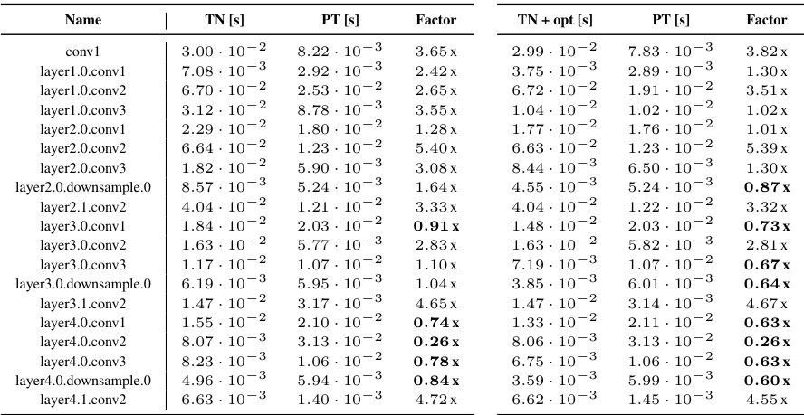
This table presents a detailed comparison of the performance of KFAC-reduce factor computation using Tensor Network (TN) and standard PyTorch implementations. It breaks down the results by different convolution types (general, mixed dense, dense, and down-sampling) and shows the TN run time, PyTorch run time, and the performance ratio (TN/PyTorch) for each convolution. The table also includes results with TN simplifications applied (TN+opt). The purpose is to demonstrate speed-ups and memory efficiencies of the TN approach, especially for less standard convolution operations.

This table presents a detailed breakdown of the performance comparison between the Tensor Network (TN) implementation and the PyTorch implementation of the input-based KFAC-reduce factor for various convolution types across different CNN architectures. It includes run times for both TN and TN+opt (TN with simplifications), along with the performance ratios (TN/PT and TN+opt/PT). The table offers a granular view of the computational gains achieved by the TN approach, particularly highlighting its efficacy for optimizing the computation of the Kronecker factor.

This table extends Table 1 from the main paper by including more operations related to convolutions. It shows the contraction strings, operands, and includes batching and channel groups. The table also describes how to generalize the operations to higher dimensions.
This table presents a comprehensive list of convolution-related operations, expanding upon Table 1 in the main paper. It details the operands and einsum contraction strings for various operations, including convolutions (with and without bias), unfolding and folding operations (im2col and col2im), Jacobian-vector products (JVPs) and vector-Jacobian products (VJPs), Kronecker-factored curvature approximations (KFC/KFAC expand and reduce), and second-order information approximations (GGN Gram matrix, Fisher/GGN diagonals). The table explicitly includes support for batching and channel groups, and indicates how the operations can be generalized to higher dimensions by extending the index notation.

This table presents a detailed breakdown of the forward pass performance for various Convolutional Neural Networks (CNNs) architectures, comparing the runtimes of Tensor Network (TN) implementations against PyTorch (PT). The results are categorized by CNN architecture and convolution type (general, dense, mixed-dense, down-sampling), providing TN runtime, PT runtime, and the performance ratio (TN/PT) for both the standard TN implementation and the optimized TN+opt implementation. Lower ratios indicate superior performance of the TN implementation.

This table provides detailed runtimes and performance factors for the forward pass of various convolutions across different CNN architectures. It compares the performance of Tensor Network (TN) and optimized TN (TN+opt) implementations against PyTorch’s built-in functionality (PT). The results are presented for various categories of convolutions: general, mixed dense, dense, and down-sampling.

This table lists the einsum contraction strings for various operations related to 2D convolutions. It shows how to express convolutions, unfolding operations (im2col), kernel unfolding (Toeplitz), vector-Jacobian products (VJPs), and Kronecker-factored curvature approximations (KFC/KFAC) using the einops library. The table includes support for batching and channel groups, and the notation is explained in the paper’s supplementary materials.

This table presents a detailed comparison of the run times for computing the input-based KFAC-reduce factor using different methods (TN, TN+opt, and PyTorch). It breaks down the performance by different convolution types (General, Mixed dense, Dense, and Down), showing the run time for each method in seconds and the performance factor (ratio of TN/TN+opt run time to PyTorch run time). This allows for a precise assessment of the computational efficiency gains achieved by using the proposed tensor network (TN) approach.

This table presents a detailed comparison of the run times and performance factors for computing the input-based KFAC-reduce factor using different methods. The comparison includes the standard PyTorch implementation (‘PT’), a Tensor Network implementation (‘TN’), and a Tensor Network implementation with simplifications (‘TN + opt’). Results are broken down by convolution type (general, mixed dense, dense, and downsampling) and for various layers within different CNN architectures (3c3d, F-MNIST 2c2d, CIFAR-100 All-CNN-C, AlexNet, ResNet18, ResNext101, and ConvNeXt-base). The ‘Factor’ column indicates the ratio of run times for each method relative to the PyTorch implementation. A factor less than 1 suggests that the TN methods are faster than the PyTorch implementation.

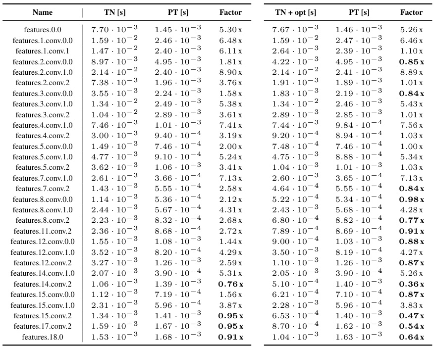
This table details the performance of KFAC-reduce factor computation using Tensor Network (TN) and standard PyTorch implementations across various CNN architectures and different convolution types (General, Mixed dense, Dense, Down). It presents the runtimes of both TN and TN+opt (with optimizations) against the PyTorch runtime (PT) and shows the performance ratios (TN/PT, TN+opt/PT) for each convolution layer. The ratios indicate speedup or slowdown compared to PyTorch. The table allows for direct comparison and analysis of the impact of Tensor Network optimizations on a key component of KFAC.

This table presents a detailed comparison of the performance of KFAC-reduce factor computation using different methods (TN, TN+opt, and PyTorch’s implementation) across various CNN architectures (3c3d, F-MNIST 2c2d, CIFAR-100 All-CNN-C, Alexnet, ResNet18, ResNext101, and ConvNeXt-base) on a GPU. For each CNN and its convolution layers, the table lists the run times in seconds for each method and calculates the performance factor (ratio of TN or TN+opt run time to PyTorch run time). The performance factor indicates the speedup or slowdown achieved by using the TN-based methods compared to the standard PyTorch implementation. Lower values indicate a greater speedup. The table also indicates the type of convolution (General, Dense mix, Dense, Down) used in each layer.

This table extends Table 1 from the main paper by including more operations related to 2D convolutions. It includes batching and channel groups and is expandable to higher dimensions. Each row describes an operation with operands, and its einsum contraction string using the einops library’s convention. The table shows the various operations the authors considered, including convolutions, Jacobian-vector products (VJPs), and Kronecker-factored approximations for curvature.
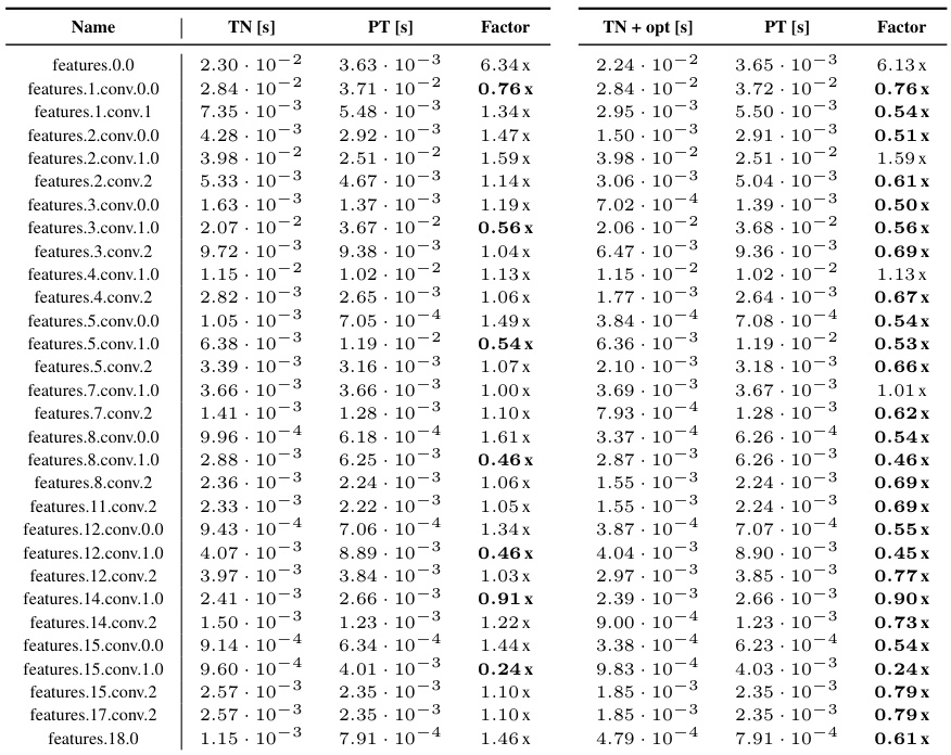
This table presents a detailed comparison of the performance of the KFAC-reduce factor computation using three different implementations: TN (Tensor Network), TN + opt (Tensor Network with optimizations), and PT (PyTorch). The results are broken down by different convolution types (General, Mixed dense, Dense, Down) across various CNN architectures and datasets. Each entry shows the run time in seconds for each implementation and the performance factor (ratio of TN or TN+opt run time to PT run time). A factor less than 1 indicates that the TN or TN+opt implementation is faster than PyTorch’s implementation.

This table presents a detailed comparison of the performance of the KFAC-reduce factor computation using Tensor Network (TN) and standard PyTorch (PT) implementations. It provides run times and performance factors (ratios of TN/PT and TN+opt/PT) for various convolution types across several different CNN architectures (3c3d, F-MNIST 2c2d, CIFAR-100 All-CNN-C, Alexnet, ResNet18, ResNext101, ConvNeXt-base). The ‘TN + opt’ column represents the performance after applying the index pattern simplifications described in the paper. The table offers a granular view of the improvements achieved by the TN approach, especially evident in the reduction of execution times and sometimes memory usage.

This table details the performance of forward pass operations (inference and training) for various CNNs. For each CNN, it shows the runtimes for the Tensor Network (TN) approach, the Tensor Network approach with optimizations (TN+opt), and the PyTorch (PT) implementation. The ‘Factor’ column shows the ratio of the TN or TN+opt runtimes to the PT runtime, indicating relative speedup or slowdown. The table helps demonstrate the efficiency of the TN approach for forward pass calculations.

This table presents a detailed comparison of the performance of KFAC-reduce factor calculations using different methods (TN and TN+opt) against a PyTorch baseline (PT). The comparison is broken down by convolution type (general, mixed dense, dense, down-sampling), and for various CNN architectures and datasets. The table shows the run times in seconds for each method and calculates performance factors indicating the relative speed of TN and TN+opt compared to PT.

This table presents a detailed comparison of the performance of the KFAC-reduce factor computation using Tensor Networks (TN) and a standard PyTorch implementation. It shows the runtimes for both TN and TN+opt (with simplifications) across different convolution types from nine CNN architectures (3c3d, F-MNIST 2c2d, CIFAR-100 All-CNN-C, AlexNet, ResNet18, ResNext101, ConvNeXt-base, Inception V3, MobileNetV2). For each convolution layer, the table lists the time taken by the TN approach and the PyTorch implementation, along with the performance ratio (Factor). The ‘Factor’ column indicates how much faster or slower the TN method is compared to the PyTorch baseline (a value <1 indicates TN is faster). The table facilitates a detailed comparison of efficiency improvements across various convolution types and network architectures.

This table presents a detailed comparison of the performance of the KFAC-reduce factor computation using Tensor Network (TN) and standard PyTorch (PT) implementations. It breaks down the results for various CNN architectures, covering general, mixed-dense, dense, and downsampling convolutions. For each convolution type, it shows the TN run time, PT run time, the performance ratio (TN/PT), the optimized TN run time (TN+opt), the optimized PT run time, and the optimized performance ratio (TN+opt/PT). The ratios indicate the speedup or slowdown achieved by using TN methods compared to standard PyTorch. A factor less than 1 signifies that the TN approach was faster.

This table presents a detailed comparison of the performance of KFAC-reduce factor computation using three different methods: the standard PyTorch implementation, the Tensor Network (TN) implementation, and the optimized Tensor Network (TN+opt) implementation. The comparison is done across various convolution types and CNN architectures, showing the runtimes (in seconds) and performance factors (ratios of runtimes) for each method. The performance factors indicate speedups or slowdowns compared to the PyTorch baseline.

This table details the performance comparison of KFAC-reduce factor calculations between the Tensor Network (TN) and standard PyTorch (PT) implementations. It shows runtimes and performance ratios (TN/PT and TN+opt/PT) for various CNN architectures (3c3d, F-MNIST 2c2d, CIFAR-100 All-CNN-C, Alexnet, ResNet18, ResNext101, ConvNeXt-base) and different convolution types within each architecture (general, mixed dense, dense, downsampling). The TN+opt column represents results where algorithmic simplifications described in the paper were applied. The ‘Factor’ column indicates the speed-up or slow-down achieved by the TN approach relative to the PT approach. The table provides a detailed view of the computational efficiency gains obtained by employing the TN approach for calculating the KFAC-reduce factor.

This table provides a comprehensive list of convolution-related operations, expanding upon Table 1 in the main paper. It details the operands and contraction strings (using the einops library convention) for various operations, including convolutions, Jacobian-vector products (JVPs), vector-Jacobian products (VJPs), Kronecker-factored approximate curvature (KFAC) calculations (both expand and reduce variants), and approximations of the generalized Gauss-Newton (GGN) matrix. The table also covers the inclusion of batching and channel groups, with a note indicating how to generalize to higher dimensions by including additional spatial and kernel indices.

This table extends Table 1 from the main paper by providing a more comprehensive list of convolution-related operations. It includes additional operations and details for hyperparameters such as batching and channel groups, extending the coverage to include a wider array of operations used in the field. The table uses the einops library’s syntax for contraction strings, making the expressions concise and readily understandable for those familiar with the library.

This table extends Table 1 from the main paper by including batching and channel groups. It lists a large number of convolution-related operations and their corresponding einsum contraction strings for implementation using the
einopslibrary. The operations cover forward and backward passes, Jacobians, VJPs, JVPs, and various curvature approximations (including KFAC and its variants). The table also demonstrates the extensibility of the approach to higher-dimensional convolutions.

This table provides an extended list of convolution and related operations, including the einsum contraction strings and operands for each operation. It expands on Table 1 from the main paper by including batching and channel groups and generalizing to higher dimensions. The table is useful for understanding the variety of operations that can be efficiently expressed using the tensor network approach.
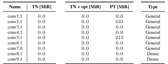
This table shows the extra memory usage beyond the memory used for input and output tensors for the computation of the KFAC-reduce factor. It compares the memory usage of the standard implementation with two versions of the tensor network implementation: one without simplifications and one with simplifications. The results are categorized by convolution type (general, dense, etc.) and show that the tensor network implementations require significantly less additional memory.

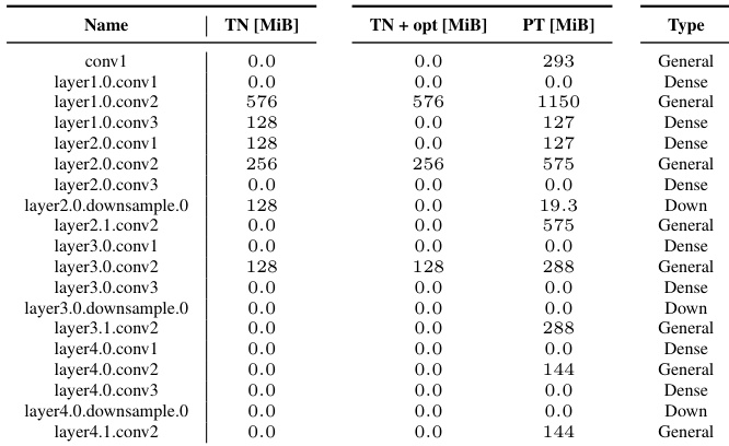
This table shows a comparison of the peak memory usage for computing the KFAC-reduce factor using three different methods: the standard PyTorch implementation, the proposed tensor network (TN) implementation, and the proposed TN implementation with simplifications. The memory usage is measured in MiB (mebibytes). The table is broken down by different convolution types found in various CNN architectures.

This table presents a comparison of the peak memory usage for different implementations of the KFAC-reduce factor calculation. The implementations are compared across various CNN architectures and convolution types (general, dense, mixed dense, downsampling). The table shows the additional memory required beyond that needed to store the input and output tensors, categorized by implementation type (TN, TN + opt, PT). A value of 0.0 indicates that the implementation uses no additional memory beyond the input and output.
This table extends Table 1 from the main paper by including more operations related to convolution, such as different types of Jacobian and VJPs, KFAC approximations, and GGN calculations. It also shows how batching and channel groups are handled. The table provides the operands and einsum contraction strings for each operation, offering a comprehensive reference for implementing various convolution-related routines.

This table shows the additional memory required to compute the KFAC-reduce factor for different CNN architectures using different implementations. The ‘TN’ column represents the Tensor Network implementation, ‘TN + opt’ is the Tensor Network implementation with optimizations, and ‘PT’ is the PyTorch implementation. A value of 0 indicates no additional memory usage beyond the input and output.

This table extends Table 1 from the main paper by including more operations and hyperparameters, such as batching and channel groups. It provides the einops contraction strings for each operation, which represent the tensor network operations in a concise notation.

This table extends Table 1 from the main paper by including additional operations related to convolutions, such as various Jacobian-vector products (JVPs), vector-Jacobian products (VJPs), and curvature approximations. The table shows the operands involved and the einsum contraction string for each operation, illustrating the flexibility and expressiveness of the einsum notation for representing these operations.
Full paper#

