Discretely beyond $1/e$: Guided Combinatorial Algortihms for Submodular Maximization

cgiOX8lfwG

Yixin Chen et el.

TL;DR
#

Submodular maximization is a critical problem in various fields, including machine learning, where the goal is to select a small subset of data points that maximize a specific function. Existing combinatorial algorithms, which are computationally efficient, were limited by an approximation ratio of 1/e, while more complex continuous methods could achieve better results. This limitation hindered practical applications.

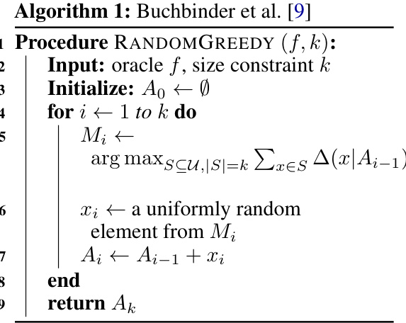
This paper presents novel combinatorial algorithms that overcome the 1/e barrier. The researchers achieved approximation ratios of 0.385 and 0.305 for size and matroid constraints respectively—higher than previously possible with combinatorial methods. These algorithms leverage a fast local search technique to guide a randomized greedy approach. Furthermore, they develop deterministic versions maintaining efficiency and performance. A deterministic nearly linear-time algorithm with a 0.377 ratio demonstrates strong practical applicability.

Key Takeaways
#

Why does it matter?
#

This paper is crucial because it significantly advances the field of submodular maximization, a vital problem in machine learning and data science. By breaking the long-standing 1/e approximation barrier for combinatorial algorithms, it offers more efficient and practical solutions for real-world applications like sensor placement and data summarization. The work also opens up new avenues of research into derandomization techniques and the exploration of nearly linear-time algorithms.

Visual Insights
#

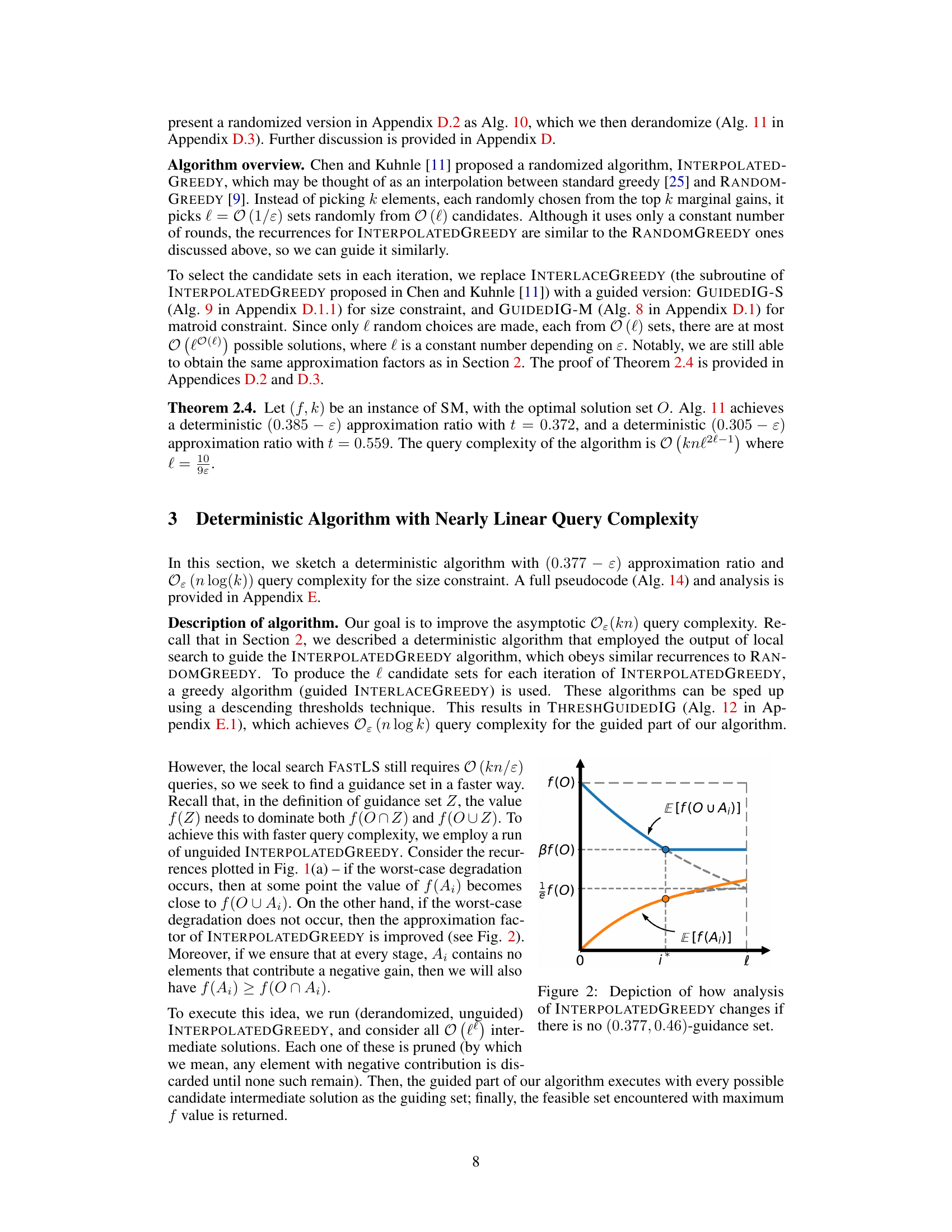
🔼 This figure shows the evolution of the expected values of f(O∪Ai) and f(Ai) in the worst-case analysis of the RANDOMGREEDY algorithm as the size of the partial solution Ai increases from 0 to k. Subfigure (a) illustrates the unguided scenario. Subfigure (b) demonstrates how the degradation of E[f(O∪Ai)] improves when using a guidance set. Subfigure (c) shows the degradation with a switch point, tk, where the algorithm initially uses guidance and then switches to an unguided approach.
read the caption
Figure 1: (a): The evolution of E [f (OU A¿)] and E [f (A¿)] in the worst case of the analysis of RANDOMGREEDY, as the partial solution size increases to k. (b): Illustration of how the degradation of E [f (OU A¿)] changes as we introduce an (0.385 + ε, 0.385)-guidance set. (c): The updated degradation with a switch point tk, where the algorithm starts with guidance and then switches to running without guidance. The dashed curved lines depict the unguided values from (a).

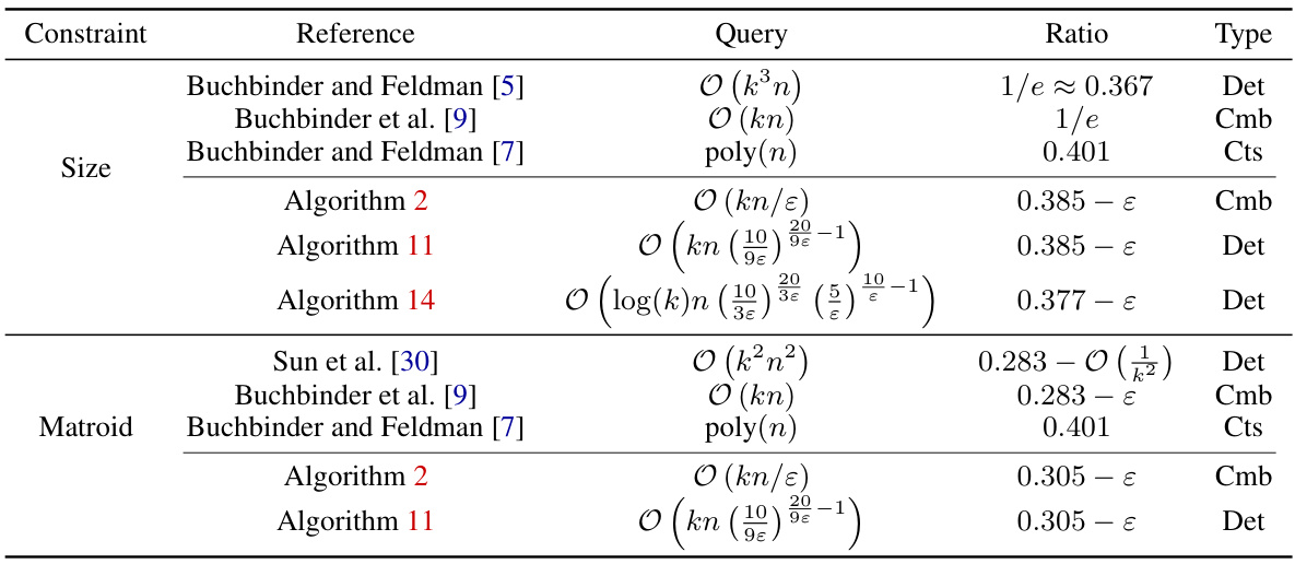
🔼 This table compares the approximation ratios achieved by different algorithms for submodular maximization problems with size and matroid constraints. It shows the query complexity, approximation ratio, and type (deterministic, randomized combinatorial, or continuous) for various algorithms. The table highlights the improvement in approximation ratio obtained by the algorithms presented in this paper compared to the prior state-of-the-art. Continuous algorithms use queries to the multilinear extension of the submodular function and its gradient, while combinatorial algorithms use only queries to the set function.
read the caption
Table 1: The prior state-of-the-art and the ratios achieved in this paper, in each category: deterministic (det), randomized combinatorial (cmb), and continuous (cts).

In-depth insights
#

Beyond 1/e Barrier
#

The research paper explores the challenge of maximizing submodular functions under constraints, a problem frequently encountered in machine learning and data science. A significant contribution lies in surpassing the well-known 1/e approximation barrier. Existing algorithms achieving ratios above 1/e often rely on continuous methods, computationally expensive to implement practically. This work focuses on combinatorial algorithms, which are more efficient for large datasets, and develops novel techniques to break the 1/e barrier for both size and matroid constraints. The key approach involves guiding a randomized greedy algorithm with results from a fast local search algorithm, improving approximation ratios and achieving deterministic versions. Achieving these improvements while maintaining reasonable computational complexity represents a substantial advancement in the field of submodular optimization, opening doors for more practical applications of these algorithms in real-world scenarios.

Guided Combinatorial
#

The concept of “Guided Combinatorial Algorithms” represents a significant advancement in submodular maximization. It intelligently blends the efficiency of combinatorial approaches with the enhanced approximation ratios typically found in continuous methods. The core idea involves guiding a combinatorial algorithm (like randomized greedy), known for its speed and simplicity, with information gleaned from a fast local search. This guidance helps the combinatorial algorithm make better choices, leading to improved approximation guarantees exceeding the 1/e barrier. The paper explores this idea in depth, providing both randomized and deterministic versions of guided algorithms, achieving ratios beyond the long-standing 1/e benchmark for both size and matroid constraints. A key contribution is the development of a fast local search technique which, surprisingly, also shows strong theoretical guarantees independently. Ultimately, “Guided Combinatorial” algorithms demonstrate a powerful paradigm for optimizing the balance between theoretical performance and practical efficiency in submodular optimization.

Deterministic Variants
#

The concept of “Deterministic Variants” in the context of submodular maximization algorithms is crucial because it addresses the inherent randomness of many high-performing algorithms. Randomized algorithms, while often achieving strong theoretical approximation ratios, can be unreliable in practice due to their stochastic nature. Their performance might vary significantly across different runs on the same input. Deterministic counterparts provide consistent results, making them more suitable for applications where reliability is paramount. The development of deterministic variants thus involves a shift in algorithmic design, likely necessitating techniques like derandomization or the use of deterministic local search procedures. Derandomization, in particular, is a complex process that might significantly increase computational cost, potentially sacrificing the efficiency of the original randomized algorithm. The trade-off between the theoretical approximation guarantees of the randomized algorithm and the practical reliability and consistent performance offered by its deterministic version is a key challenge. Achieving comparable approximation ratios while maintaining the deterministic property is therefore a major contribution. Finally, the analysis of deterministic variants must be rigorous, demonstrating that the approximation bounds hold deterministically, which can be more challenging than the analysis of randomized counterparts.

Nearly Linear Time
#

The concept of “Nearly Linear Time” in the context of submodular maximization is significant because it addresses a critical limitation of existing algorithms. Many algorithms that achieve approximation ratios beyond the 1/e barrier rely on continuous methods, which are computationally expensive. A nearly linear time algorithm offers a practical solution, bridging the gap between theoretical advancements and real-world applicability. This is achieved by carefully designing a deterministic algorithm that guides a greedy approach with a fast local search. The focus is on reducing query complexity, which translates to faster computation times, especially crucial when dealing with large datasets. The success hinges on achieving a near-linear time complexity without sacrificing the approximation ratio, a significant contribution to the field. This work highlights the practical implications of improving algorithmic efficiency for constrained submodular maximization problems.

Empirical Evaluation
#

The empirical evaluation section of a research paper is crucial for validating theoretical claims. A strong empirical evaluation should compare the proposed method against relevant baselines on multiple datasets. Objective metrics should be used to quantify the performance, and statistical significance should be assessed. The paper should clearly explain the experimental setup, including details on the datasets used, any preprocessing steps, and hyperparameter tuning strategies. Visualization of results through graphs and tables helps readers easily understand the performance comparison. The results should be discussed in detail, highlighting the strengths and weaknesses of the proposed method. The empirical evaluation should justify the claims made in the introduction and conclude whether the proposed method significantly improves upon existing techniques. Reporting runtime and query complexity is also vital, as it helps assess the practical feasibility and efficiency of the proposed method.

More visual insights
#

More on figures

🔼 This figure illustrates the evolution of the expected values of f(O∪A;) and f(A;) in the analysis of the RANDOMGREEDY algorithm, as the size of the partial solution increases to k. It compares the worst-case scenario of the original algorithm with the improved degradation achieved by incorporating a guidance set. The figure shows how the guidance set improves the algorithm’s performance by reducing the degradation of E[f(O∪A;)] and improving the overall approximation ratio.
read the caption
Figure 1: (a): The evolution of E[f(O∪A;)] and E[f(A;)] in the worst case of the analysis of RANDOMGREEDY, as the partial solution size increases to k. (b): Illustration of how the degradation of E[f(O∪A;)] changes as we introduce an (0.385+ε, 0.385)-guidance set. (c): The updated degradation with a switch point tk, where the algorithm starts with guidance and then switches to running without guidance. The dashed curved lines depict the unguided values from (a).

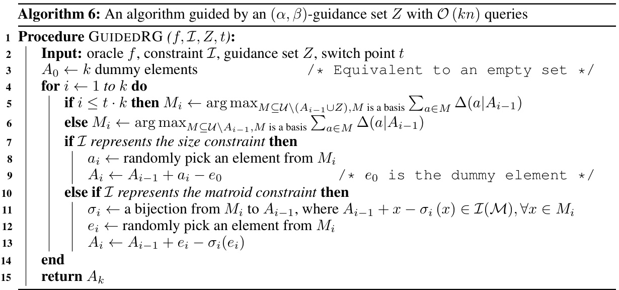
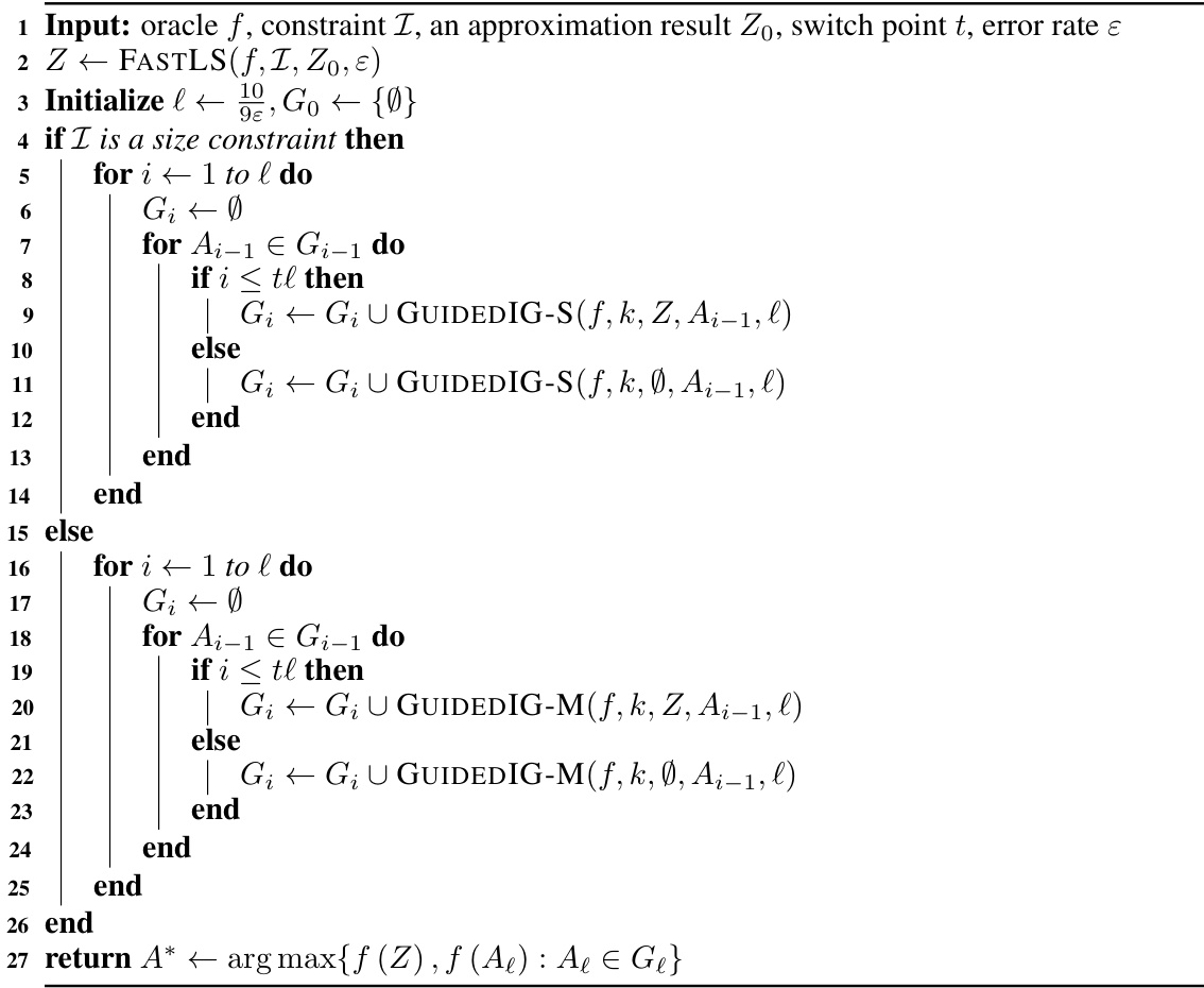
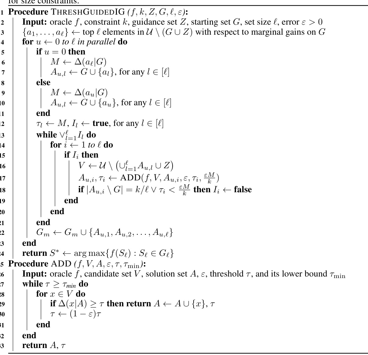
🔼 This figure compares the performance of the proposed algorithm (FASTLS+GUIDEDRG) against three baselines: STANDARDGREEDY, RANDOMGREEDY, and the algorithm by Lee et al. The performance is measured in terms of objective value (higher is better) and the number of queries (lower is better), both normalized by those of STANDARDGREEDY. The results are shown for two different applications of size-constrained submodular maximization (video summarization and maximum cut), and for varying values of k/n (the ratio of the constraint size k to the size of the ground set n). The plots illustrate that the proposed algorithm often achieves a higher objective value than the baselines, especially in the maximum cut experiments, while maintaining a relatively low query complexity.
read the caption
Figure 3: The objective value (higher is better) and the number of queries (log scale, lower is better) are normalized by those of STANDARDGREEDY. Our algorithm (blue star) outperforms every baseline on at least one of these two metrics.

🔼 This figure shows the analysis of the RANDOMGREEDY algorithm’s performance in the worst-case scenario. Subfigure (a) illustrates how the expected values of the objective function (f(OU A¿)) and the selected set’s value (f(A¿)) change as the algorithm progresses. Subfigure (b) demonstrates the improvement achieved by introducing a guidance set, reducing the degradation of the objective function’s expected value. Finally, subfigure (c) shows the combined effect of both guidance and a switch point, resulting in a better approximation ratio.
read the caption
Figure 1: (a): The evolution of E[f(OU A¿)] and E[f(A¿)] in the worst case of the analysis of RANDOMGREEDY, as the partial solution size increases to k. (b): Illustration of how the degradation of E[f(OU A¿)] changes as we introduce an (0.385 + ε, 0.385)-guidance set. (c): The updated degradation with a switch point tk, where the algorithm starts with guidance and then switches to running without guidance. The dashed curved lines depict the unguided values from (a).

🔼 This figure shows the behavior of the expected values of the objective function f(A) and f(O∪A) for RANDOMGREEDY, where A is the current solution and O is the optimal solution. Subfigure (a) depicts the worst-case scenario for the unguided algorithm, showing how f(A) converges to OPT/e. Subfigures (b) and (c) illustrate how a guidance set improves this behavior by reducing the degradation of f(O∪A) and ultimately leading to a better approximation ratio. The switch point tk represents the point where the algorithm transitions from guided to unguided behavior.
read the caption
Figure 1: (a): The evolution of E [f (OU A¿)] and E [f (A¿)] in the worst case of the analysis of RANDOMGREEDY, as the partial solution size increases to k. (b): Illustration of how the degradation of E [f (OU A¿)] changes as we introduce an (0.385 + ε, 0.385)-guidance set. (c): The updated degradation with a switch point tk, where the algorithm starts with guidance and then switches to running without guidance. The dashed curved lines depict the unguided values from (a).

🔼 This figure illustrates the behavior of the expected values of f(Aᵢ) (the value of the solution built by RANDOMGREEDY) and f(O∪Aᵢ) (the value of the optimal solution combined with the partial solution built by RANDOMGREEDY) as the algorithm progresses. Panel (a) shows the classical RANDOMGREEDY analysis where both converge to OPT/e. Panel (b) shows the improvement gained by introducing a guidance set; the curves show less degradation. Panel (c) shows that further improvement is possible by employing a hybrid approach—using a guidance set early on and then switching to the unguided RANDOMGREEDY.
read the caption
Figure 1: (a): The evolution of E[f(O∪Aᵢ)] and E[f(Aᵢ)] in the worst case of the analysis of RANDOMGREEDY, as the partial solution size increases to k. (b): Illustration of how the degradation of E[f(O∪Aᵢ)] changes as we introduce an (0.385+ε, 0.385)-guidance set. (c): The updated degradation with a switch point tk, where the algorithm starts with guidance and then switches to running without guidance. The dashed curved lines depict the unguided values from (a).

🔼 This figure shows the evolution of the expected values of the objective function f(A;) and its intersection with the optimal solution f(O∪A;) for the RANDOMGREEDY algorithm. Subfigure (a) illustrates the standard RANDOMGREEDY behavior, showing a gradual convergence towards OPT/e. Subfigure (b) demonstrates how the introduction of a guidance set improves the degradation of E[f(O∪A;)], leading to better gains. Subfigure (c) shows how the algorithm starts with guidance and then switches to unguided behavior at a switch point tk, effectively combining the benefits of both approaches for better approximation.
read the caption
Figure 1: (a): The evolution of E[f(O∪A;)] and E[f(A;)] in the worst case of the analysis of RANDOMGREEDY, as the partial solution size increases to k. (b): Illustration of how the degradation of E[f(O∪A;)] changes as we introduce an (0.385+ε, 0.385)-guidance set. (c): The updated degradation with a switch point tk, where the algorithm starts with guidance and then switches to running without guidance. The dashed curved lines depict the unguided values from (a).

🔼 This figure illustrates the performance of the RANDOMGREEDY algorithm with and without guidance. Subfigure (a) shows the standard degradation of the expected objective function value as the algorithm progresses. Subfigure (b) demonstrates the improved degradation when a guidance set is used. Subfigure (c) shows how switching between guided and unguided phases can further improve performance.
read the caption
Figure 1: (a): The evolution of E[f(O∪Ai)] and E[f(Ai)] in the worst case of the analysis of RANDOMGREEDY, as the partial solution size increases to k. (b): Illustration of how the degradation of E[f(O∪Ai)] changes as we introduce an (0.385+ε, 0.385)-guidance set. (c): The updated degradation with a switch point tk, where the algorithm starts with guidance and then switches to running without guidance. The dashed curved lines depict the unguided values from (a).

🔼 This figure shows the evolution of the expected values of f(O∪A;) and f(A;) in the worst-case analysis of the RANDOMGREEDY algorithm. Panel (a) shows the unguided case, demonstrating the convergence to OPT/e. Panel (b) illustrates how introducing a guidance set improves the degradation of E[f(O∪A;)], leading to better gains later in the algorithm. Finally, panel (c) shows the updated degradation using a switch point (tk) to combine the benefits of both guided and unguided approaches.
read the caption
Figure 1: (a): The evolution of E[f(O∪A;)] and E[f(A;)] in the worst case of the analysis of RANDOMGREEDY, as the partial solution size increases to k. (b): Illustration of how the degradation of E[f(O∪A;)] changes as we introduce an (0.385+ε, 0.385)-guidance set. (c): The updated degradation with a switch point tk, where the algorithm starts with guidance and then switches to running without guidance. The dashed curved lines depict the unguided values from (a).

🔼 This figure compares the frames selected by FASTLS+GUIDEDRG and STANDARDGREEDY algorithms for video summarization. The top row shows the frames selected by FASTLS+GUIDEDRG, and the bottom row shows the frames selected by STANDARDGREEDY. The figure visually demonstrates the difference in frame selection between the two algorithms.
read the caption
Figure 5: Frames selected for Video Summarization

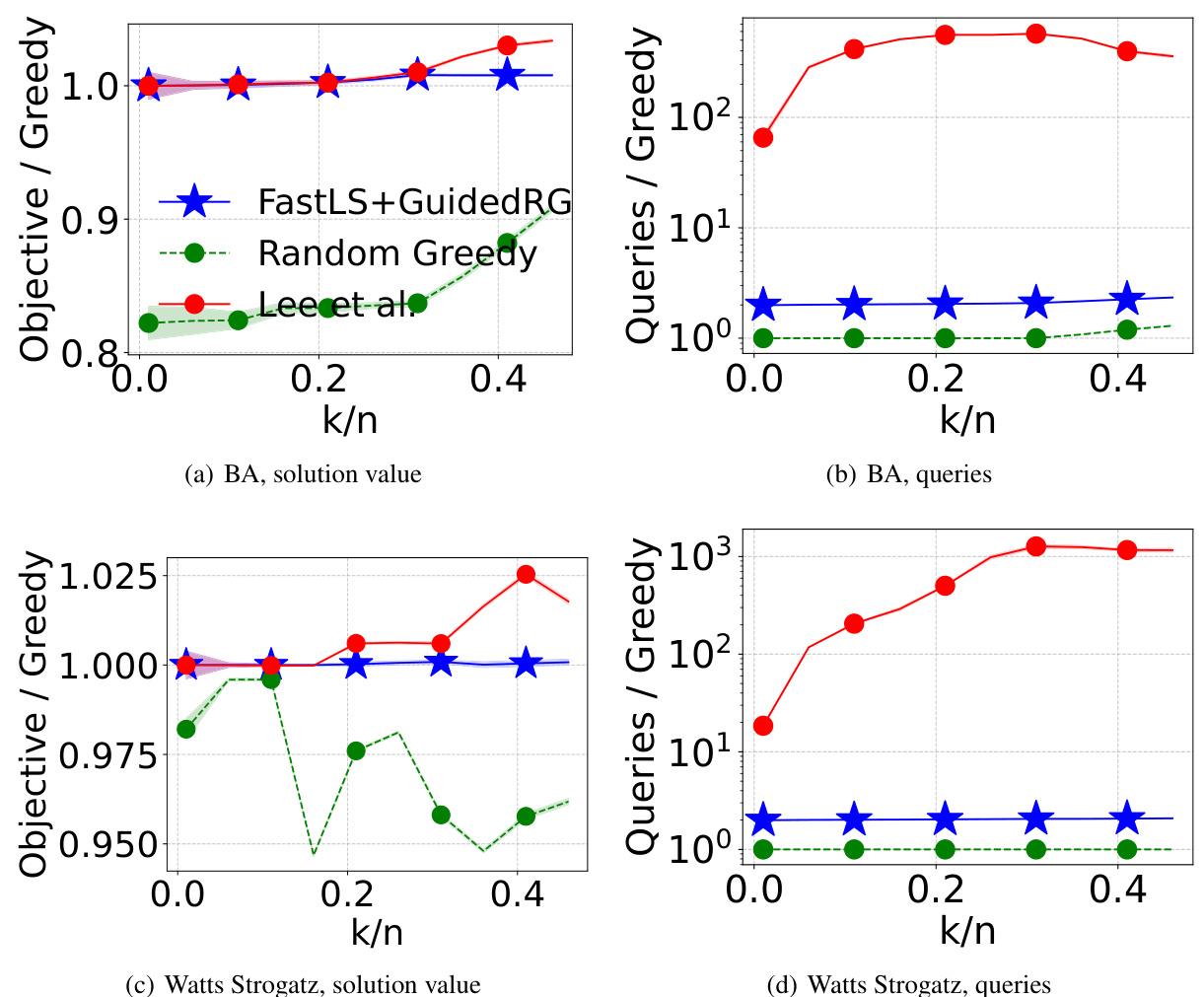
🔼 This figure compares the performance of the proposed FASTLS+GUIDEDRG algorithm against three baselines: STANDARDGREEDY, RANDOMGREEDY, and the algorithm by Lee et al. The comparison is made across two applications of size-constrained submodular maximization: video summarization and maximum cut. For each application, two plots are shown: one for the objective value (normalized by STANDARDGREEDY) and one for the number of queries (also normalized by STANDARDGREEDY). The results indicate that FASTLS+GUIDEDRG consistently outperforms or matches the baselines in terms of objective value while maintaining comparable query counts, especially with increasing k/n (ratio of the size constraint to the size of the ground set).
read the caption
Figure 3: The objective value (higher is better) and the number of queries (log scale, lower is better) are normalized by those of STANDARDGREEDY. Our algorithm (blue star) outperforms every baseline on at least one of these two metrics.

TL;DR#

Key Takeaways#

Why does it matter?#

Visual Insights#

In-depth insights#

Beyond 1/e Barrier#

Guided Combinatorial#

Deterministic Variants#

Nearly Linear Time#

Empirical Evaluation#

More visual insights#

Full paper#