TL;DR#
Training neural networks often involves gradient descent (GD). While theoretical analyses typically focus on small stepsizes leading to monotonic risk reduction, large stepsizes used in practice lead to initial risk oscillations before monotonic decrease. This discrepancy has hampered a full understanding of GD’s behavior. Existing studies fail to address this issue, especially in the context of complex, non-homogeneous neural networks.
This research investigates large stepsize GD in non-homogeneous two-layer networks. The authors demonstrate that after an initial oscillating phase, the empirical risk decreases monotonically, and network margins grow nearly monotonically, showing an implicit bias of GD. Importantly, they show that large stepsize GD, incorporating the two-phased behavior, is more efficient than small stepsize GD under suitable conditions, extending theory beyond simplified setups.
Key Takeaways#
Why does it matter?#
This paper is crucial for researchers in deep learning optimization because it bridges the gap between theoretical understanding and practical applications of large-stepsize gradient descent (GD). It provides insights into the dynamics of GD for neural networks beyond simplified linear models. By exploring the behavior of large-stepsize GD in the context of non-homogeneous networks, the paper offers new theoretical tools for understanding implicit bias, optimization efficiency, and generalization performance. This is particularly relevant in light of the widespread use of large stepsizes in practical deep learning applications.
Visual Insights#

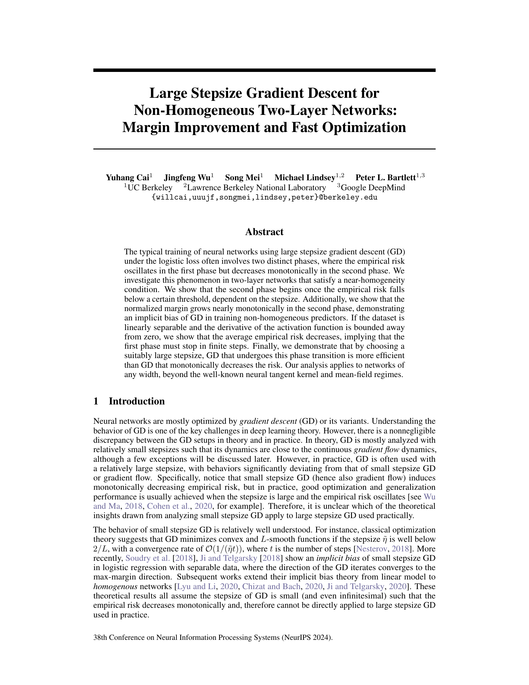
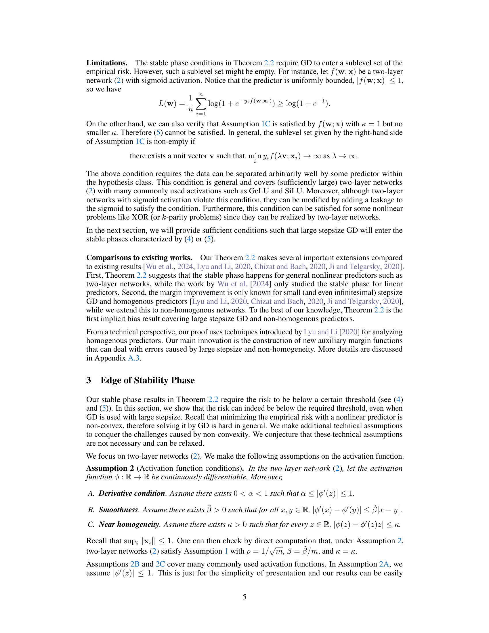
🔼 This figure shows the training dynamics of a four-layer MLP using gradient descent (GD) with different step sizes on a subset of the CIFAR-10 dataset. It illustrates the two-phase training behavior often observed with large stepsize GD: an initial oscillatory phase followed by a monotonic decrease in empirical risk. The figure compares large and small stepsizes, highlighting how the large stepsize leads to faster convergence and improved test accuracy, while both step sizes show a similar monotonic increase in normalized margin during the second phase of training.
read the caption
Figure 1: The behavior of (GD) for optimizing a non-homogenous four-layer MLP with GELU activation function on a subset of CIFAR-10 dataset. We randomly sample 6,000 data with labels “airplane” and “automobile” from CIFAR-10 dataset. The normalized margin is defined as mini∈[n] Yif (wt; xi)/||wt||4, which is close to (3). The blue curves correspond to GD with a large stepsize ที = 0.2, where the empirical risk oscillates in the first phase but decreases monotonically in the second phase. The orange curves correspond to GD with a small stepsize ῆ = 0.005, where the empirical risk decreases monotonically. Furthermore, Figure 1(b) suggests the normalized margins of both two curves increase and converge in the stable phases. Finally, Figure 1(c) suggests that large stepsize achieves a better test accuracy, consistent with larger-scale learning experiment [Hoffer et al., 2017, Goyal et al., 2017].
In-depth insights#
Large Stepsize GD#
The study explores the dynamics of large stepsize gradient descent (GD) in training neural networks, particularly focusing on two-layer networks. A key finding is the identification of two distinct phases during training: an initial phase where empirical risk oscillates, followed by a stable phase with monotonic risk decrease. This transition occurs once the empirical risk drops below a stepsize-dependent threshold. The analysis reveals that the normalized margin grows nearly monotonically in the second phase, indicating an implicit bias of GD towards maximizing margins, even in non-homogeneous networks. Importantly, the research demonstrates that, with a suitably large stepsize, GD is more efficient than its small stepsize counterpart, achieving a faster convergence rate while minimizing the risk. The results extend the understanding of GD beyond the commonly studied small stepsize and mean-field regimes, offering valuable insights into the practical optimization of neural networks.
Stable Phase Bias#
The concept of “Stable Phase Bias” in the context of large stepsize gradient descent for neural network training is a compelling area of research. It suggests that the seemingly chaotic initial phase of training, where the empirical risk fluctuates, eventually transitions to a stable phase characterized by monotonic risk decrease. This transition is not merely a consequence of the optimization algorithm converging towards a minimum but, rather, an emergent property potentially tied to an implicit bias that favors certain solutions. Understanding this bias is crucial as it could explain the generalization performance observed in practice despite the non-convex nature of the loss landscape. Further investigation is needed to fully characterize this bias, considering factors like network architecture, activation functions, and data properties. Determining whether this stable phase bias is fundamentally linked to max-margin solutions or represents a more general phenomenon warrants further study. The existence of this bias could also have significant implications for algorithm design and hyperparameter tuning, as it may provide a theoretical basis for choosing optimal step sizes and for potentially guiding the search for efficient training strategies. Ultimately, unravelling the mysteries of the stable phase and its underlying bias will lead to a more profound comprehension of deep learning’s successes.
Non-Convex Loss#
The concept of a non-convex loss function is central to many machine learning problems, particularly those involving neural networks. Non-convexity introduces challenges in optimization, as gradient descent methods may converge to local minima instead of the global optimum, leading to suboptimal performance. However, the same non-convexity can also be a source of strength. Recent research suggests that the implicit bias of gradient descent in non-convex landscapes can lead to surprisingly good generalization, even when the empirical risk is not fully minimized. Understanding this interplay between optimization difficulty and generalization capability is a key focus of modern machine learning research. The choice of loss function and the optimization algorithm significantly impact the final model’s properties, including its bias, variance, and robustness to noisy data or adversarial examples. Therefore, analyzing the effects of non-convex loss functions requires a thorough understanding of both the optimization process and the properties of the resulting model. The ability to handle non-convexity is crucial in dealing with high-dimensional data and complex relationships. Further exploration of specific non-convex loss functions, such as those based on cross-entropy or other specialized metrics, offers valuable opportunities for advancing our understanding of model behavior and improving predictive accuracy.
Margin Improvement#
The concept of “Margin Improvement” in the context of large stepsize gradient descent for training neural networks is a crucial finding. It demonstrates that despite the oscillations observed in the empirical risk during the initial training phase, the normalized margin, a measure of the classifier’s confidence, grows nearly monotonically once the training enters a stable phase. This implies that even with large stepsizes, which deviate significantly from the behavior of gradient flow, the algorithm exhibits an implicit bias towards maximizing the margin. This implicit bias is particularly important because it suggests that the algorithm is not simply memorizing the data but is instead learning a more generalizable representation. The margin improvement is not limited to linearly separable data or homogenous networks, signifying a broader applicability of this behavior. The analysis extends prior work which focused on small stepsize gradient descent, revealing novel insights into the optimization dynamics of large stepsize algorithms often used in practice. This discovery is a significant theoretical contribution to our understanding of implicit bias, helping us bridge the gap between theory and practice in deep learning.
Fast Optimization#
The heading ‘Fast Optimization’ likely discusses how the proposed method achieves faster convergence compared to traditional gradient descent. The authors probably demonstrate that large step sizes, while initially causing oscillations in the empirical risk, ultimately lead to faster risk reduction in the stable phase. This is a crucial finding as it challenges the conventional wisdom of using small step sizes for GD. The analysis likely compares the convergence rate (e.g., O(1/t²) vs O(1/t)) of large vs. small step size GD, showing a significant speedup in optimization for the former. Theoretical bounds on the number of steps required to reach a certain risk level are presented, potentially showing the superiority of the proposed method for large-scale learning scenarios. Empirical results visualizing faster training curves with large step sizes are probably also presented to support this claim. This section is critical as it offers practical advice and justifies the use of larger step sizes, which are often employed in practice but lack strong theoretical justification.
More visual insights#
More on figures

🔼 This figure shows the training dynamics of a four-layer MLP on a subset of CIFAR-10 using gradient descent (GD) with different step sizes. The plots illustrate the empirical risk, normalized margin, and test accuracy over training iterations. The key observation is that a larger step size leads to an initial oscillatory phase in the empirical risk, followed by a monotonic decrease, while a smaller step size results in a consistently monotonic decrease. Despite the initial oscillations, the larger step size achieves a better test accuracy and a similar final normalized margin as the smaller step size.
read the caption
Figure 1: The behavior of (GD) for optimizing a non-homogenous four-layer MLP with GELU activation function on a subset of CIFAR-10 dataset. We randomly sample 6,000 data with labels “airplane” and “automobile” from CIFAR-10 dataset. The normalized margin is defined as mini∈[n] Yif (wt; xi)/||wt||4, which is close to (3). The blue curves correspond to GD with a large stepsize ที = 0.2, where the empirical risk oscillates in the first phase but decreases monotonically in the second phase. The orange curves correspond to GD with a small stepsize ῆ = 0.005, where the empirical risk decreases monotonically. Furthermore, Figure 1(b) suggests the normalized margins of both two curves increase and converge in the stable phases. Finally, Figure 1(c) suggests that large stepsize achieves a better test accuracy, consistent with larger-scale learning experiment [Hoffer et al., 2017, Goyal et al., 2017].

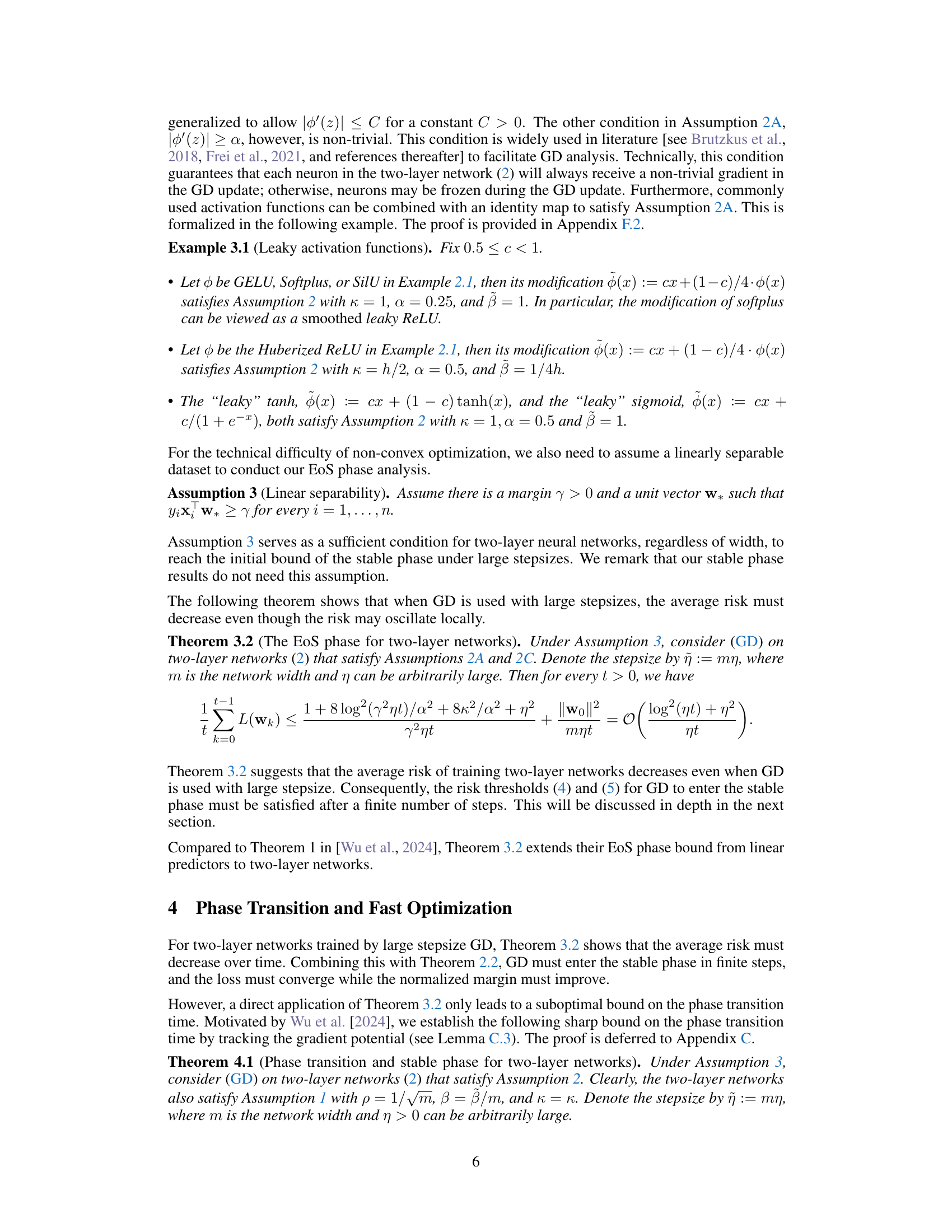
🔼 Figure 2 displays the results of experiments conducted on two-layer neural networks with leaky softplus activation. Two datasets are used: a synthetic XOR dataset and a subset of CIFAR-10. The plots show the empirical risk, asymptotic convergence rate, and normalized margin for different step sizes of Gradient Descent (GD). The results demonstrate that larger step sizes lead to faster optimization, an asymptotic convergence rate of O(1/(ῆt)), and a nearly monotonically increasing normalized margin during the stable phase, aligning with the paper’s theoretical analysis.
read the caption
Figure 2: Behavior of (GD) for two-layer networks (2) with leaky softplus activation function (see Example 3.1 with c = 0.5). We consider an XOR dataset and a subset of CIFAR-10 dataset. In both cases, we observe that (1) GD with a large stepsize achieves a faster optimization compared to GD with a small stepsize, (2) the asymptotic convergence rate of the empirical risk is O(1/(ῆt)), and (3) in the stable phase, the normalized margin (nearly) monotonically increases. These observations are consistent with our theoretical understanding of large stepsize GD. More details about the experiments are explained in Section 5.

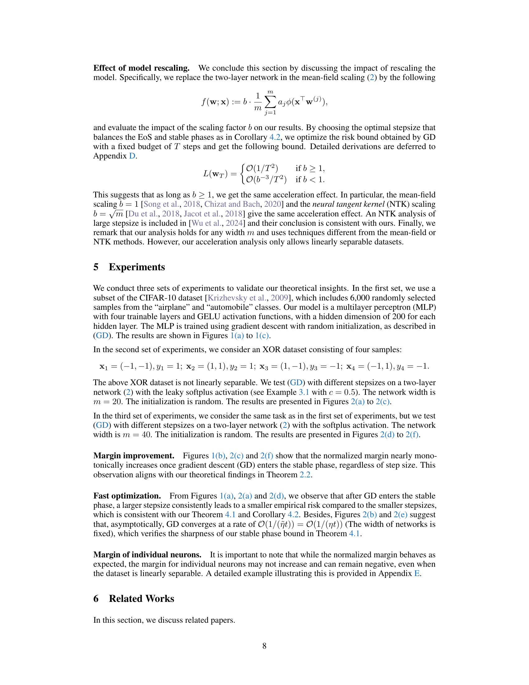
🔼 The figure shows the empirical risk, asymptotic convergence rate, and normalized margin for gradient descent (GD) using different step sizes on two-layer neural networks. The experiments were performed on an XOR dataset and a subset of the CIFAR-10 dataset. The results demonstrate that using a large step size leads to faster optimization and a nearly monotonically increasing normalized margin in the stable phase, which is consistent with the theoretical findings.
read the caption
Figure 2: Behavior of (GD) for two-layer networks (2) with leaky softplus activation function (see Example 3.1 with c = 0.5). We consider an XOR dataset and a subset of CIFAR-10 dataset. In both cases, we observe that (1) GD with a large stepsize achieves a faster optimization compared to GD with a small stepsize, (2) the asymptotic convergence rate of the empirical risk is O(1/(ῆt)), and (3) in the stable phase, the normalized margin (nearly) monotonically increases. These observations are consistent with our theoretical understanding of large stepsize GD. More details about the experiments are explained in Section 5.
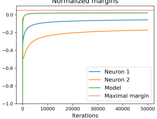
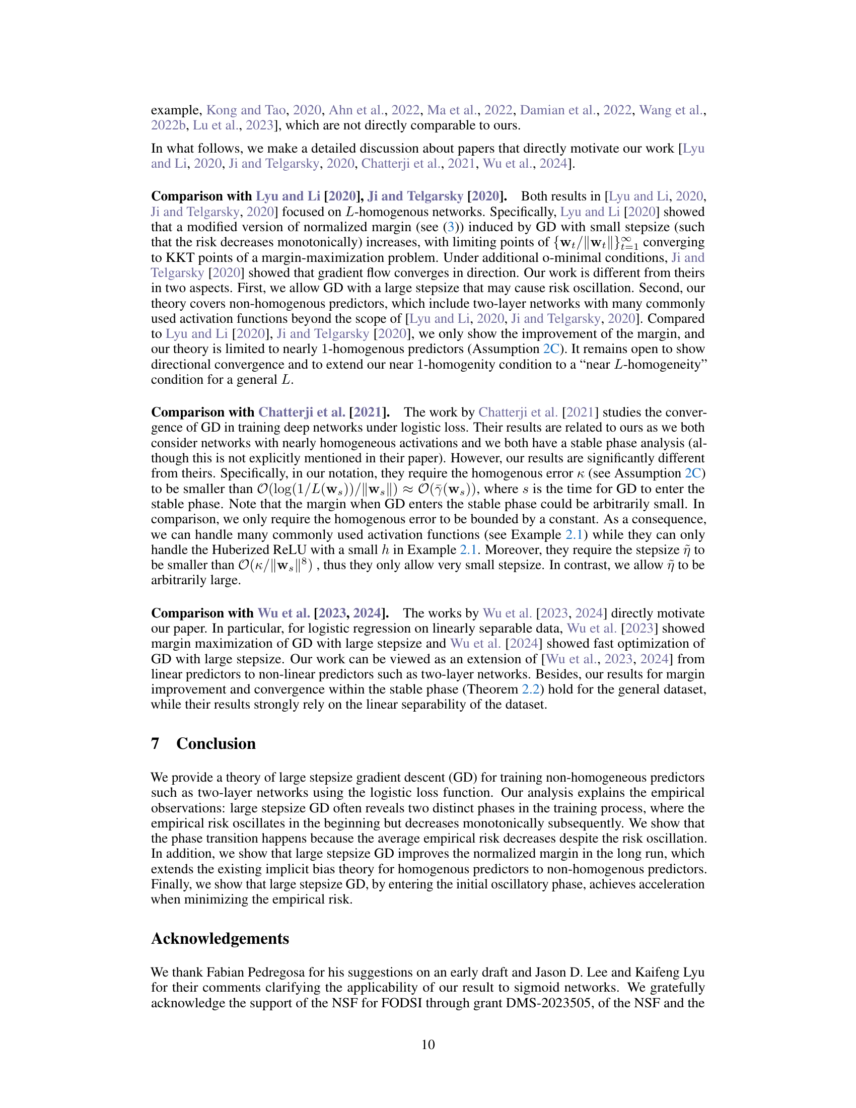
🔼 The figure shows training loss and normalized margins for a two-layer neural network with leaky softplus activation trained on a synthetic dataset. Despite individual neurons having negative margins, the overall network margin increases and becomes positive, illustrating the model’s behavior even with non-monotonic risk.
read the caption
Figure 4: Training loss and margins of a two-layer network with leaky softplus activations on a synthetic linear separable dataset. There are five samples in the dataset, which are ((0.05, 1, 2), 1), ((0.05, −2, 1), 1), ((−1, 0, 2), −1), ((0.05, -2, -2), 1), ((0.05, 1, -2), 1). The max margin direction is (1,0,0) with a normalized margin of 0.05. The network only has two neurons with fixed weights 1/2 and -1/2. The leaky softplus activation is f(x) = (x + ¢(x))/2, where ∮ is the softplus activation. The stepsize is 3. We can observe that both neurons have negative margins during the training, while the network's margin increases and becomes positive.
Full paper#
