TL;DR#
Stochastic bandits struggle with large action spaces. Existing approaches use linear models, kernel regression, or neural networks to model reward, but their effectiveness depends on the reward model’s accuracy. Tree ensembles offer a potentially better reward estimation model, but their use in bandits is underexplored. Neural networks are also limited by super-linear regret growth.
This paper proposes a novel bandit algorithm (ST-UCB) that uses soft tree ensemble models. By analyzing the soft tree properties, they extend analytical techniques from neural bandit algorithms. ST-UCB demonstrates lower cumulative regret than existing ReLU-based neural bandit algorithms, but with a more constrained hypothesis space. This provides a theoretical foundation for using tree ensembles in stochastic bandits, addressing existing limitations of other methods.
Key Takeaways#
Why does it matter?#
This paper is important as it bridges the gap between tree-based models and the theoretical framework of neural bandits offering a novel algorithm with improved regret bounds. This opens avenues for research combining the strengths of both approaches, potentially leading to more efficient and robust bandit algorithms.
Visual Insights#
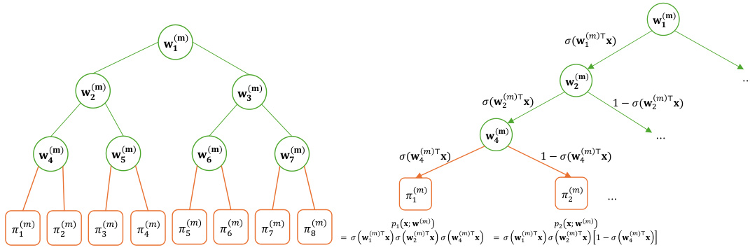
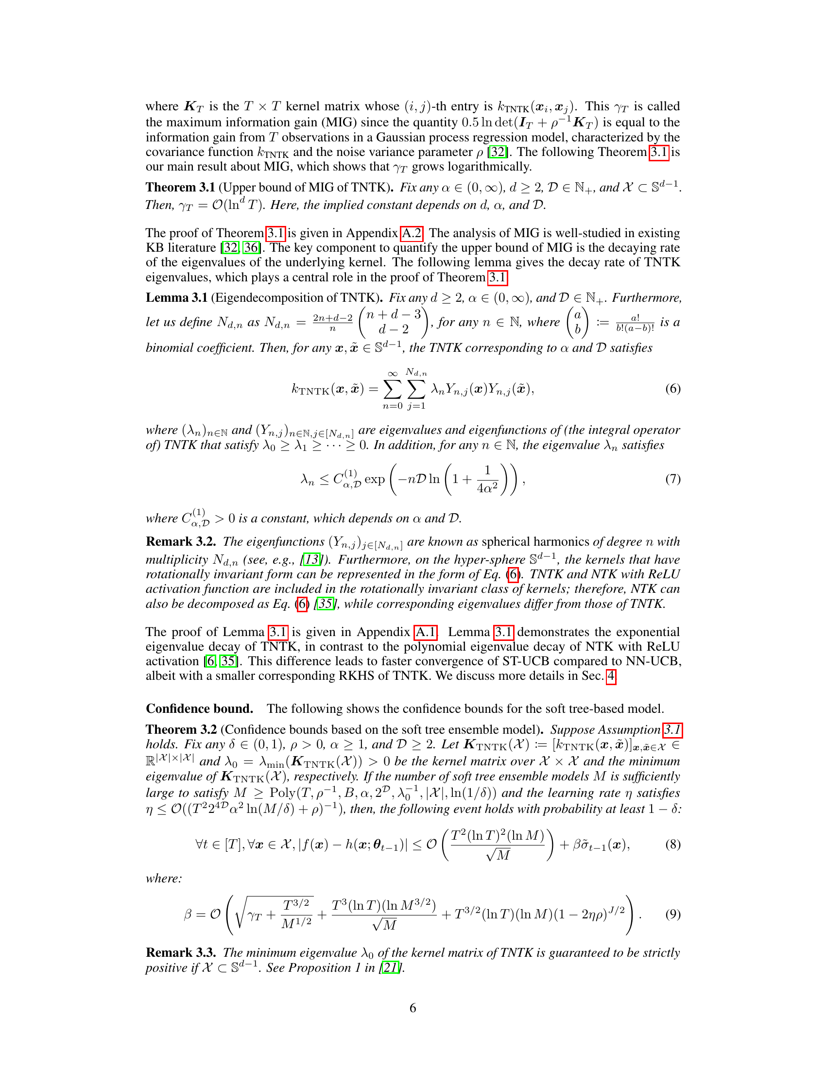
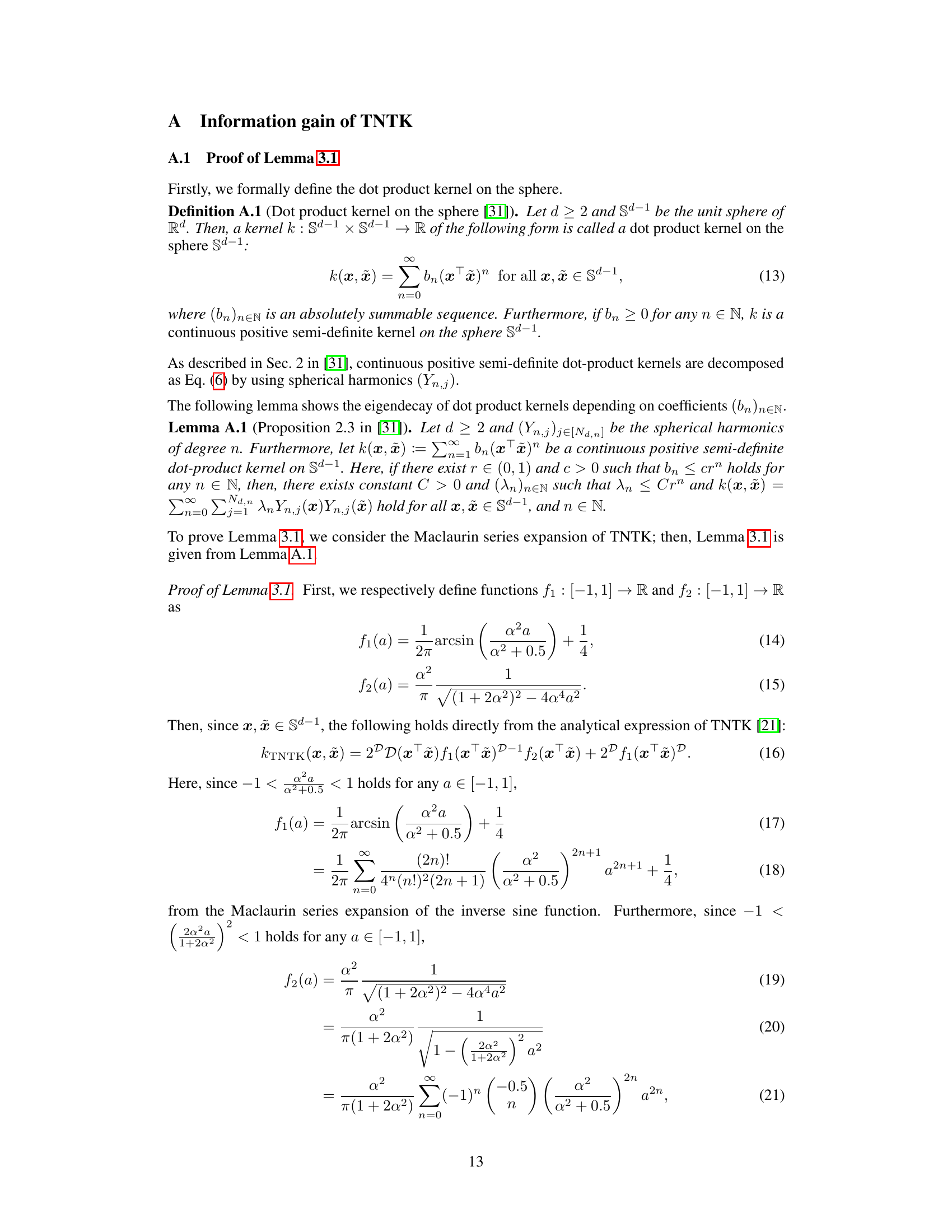
🔼 This figure illustrates the structure of a soft tree with depth D=3. The left plot shows the tree structure with internal nodes (green) and leaf nodes (orange) labeled using breadth-first ordering. The number of internal nodes is N = 2D -1 and the number of leaf nodes is L = 2D. The right plot demonstrates how a soft tree computes the weight probabilities for each leaf node using the soft decision function.
read the caption
Figure 1: An illustrative image of a soft tree structure with D = 3. As shown in the left plot, we have N := 2D − 1 internal nodes (green) and L := 2D leaf nodes (orange), indexed using breadth-first ordering. The right plot shows an illustrative example where a soft tree calculates the weight probabilities pι(·) for the leaf nodes.
In-depth insights#
Soft Tree Bandit#
The concept of a ‘Soft Tree Bandit’ blends the advantages of soft tree models with the exploration-exploitation framework of bandit algorithms. Soft tree models, unlike traditional decision trees, employ a gradient-based approach to learn decision boundaries, resulting in smoother and more robust predictions. This smoothness is crucial in bandit settings, where accurate reward estimations are essential to guide exploration. By using a soft tree as the underlying model, the resulting ‘Soft Tree Bandit’ algorithm can potentially achieve lower regret compared to algorithms using hard decision trees or other simpler reward models, such as linear bandits. This is because the softer boundaries help to better capture complex relationships between contexts and rewards, reducing the risk of overfitting. However, the hypothesis space of soft tree ensemble models is inherently more constrained than that of neural networks, representing a trade-off between model expressiveness and regret bounds. Therefore, a ‘Soft Tree Bandit’ offers an interesting middle ground, providing a balance between practical performance and theoretical guarantees.
Regret Analysis#
Regret analysis in the context of bandit algorithms is crucial for evaluating the performance of exploration-exploitation strategies. It quantifies the difference between the cumulative reward obtained by an algorithm and that of an optimal strategy that always selects the best action. The core of regret analysis lies in establishing upper bounds on the cumulative regret, ideally demonstrating that this regret grows sublinearly with the number of time steps. This sublinear growth ensures a ’no-regret’ property, meaning the average per-step regret vanishes as time progresses. Different structural assumptions on the reward function impact the achievable regret bounds. For example, linear or Lipschitz assumptions on rewards allow for tighter regret bounds compared to more general settings. The analysis often involves concentration inequalities, martingale arguments, and reproducing kernel Hilbert spaces (RKHS). The techniques used for regret analysis vary depending on the underlying model used to estimate rewards (linear, kernel, or neural networks). The paper’s analysis likely incorporates the neural tangent kernel (NTK) theory, a powerful tool for analyzing overparameterized neural networks, to derive regret bounds for the soft tree-based algorithm. A key aspect is establishing the complexity of the hypothesis space of the reward estimation model, and how this impacts the resulting regret. The trade-off between model capacity and regret is a major consideration. A more constrained model with a smaller hypothesis space (like soft trees) may lead to lower regret than a more complex model but only under specific assumptions.
Hypothesis Space#
The concept of ‘hypothesis space’ in the context of bandit algorithms is crucial. It represents the set of all possible reward functions the algorithm can learn. The paper highlights a key trade-off: the soft tree ensemble model offers a more constrained hypothesis space compared to the commonly used ReLU-based neural networks. This constraint, while seemingly limiting, leads to a significant advantage. The reduced complexity helps the algorithm avoid overfitting and achieve a better regret bound (Õ(√T)) even in general action spaces. Unlike neural networks, the soft tree-based approach provides a consistent no-regret guarantee without needing restrictive assumptions on the action space. The paper suggests that this advantage is likely due to the inherent structural regularisation of soft trees, and implies that the choice of the soft decision function within the soft tree model also plays an important role in shaping the hypothesis space and overall regret performance. Further investigation into non-smooth soft-decision functions could potentially bridge the gap between the hypothesis spaces of the two model types.
Empirical Results#
An Empirical Results section for this research paper would ideally present a detailed comparison of the proposed soft tree-based UCB (ST-UCB) algorithm against existing methods like neural UCB (NN-UCB) and e-greedy variants. Key performance metrics would include cumulative regret, showcasing ST-UCB’s superior performance across various datasets (real-world and synthetic) and reward functions. The analysis should delve into the impact of hyperparameters and the algorithm’s robustness to different settings. Visualizations, such as plots showing cumulative regret over time for each algorithm, would be crucial for clear interpretation. Statistical significance tests should be used to validate the observed differences in performance. A discussion on the trade-offs between ST-UCB and NN-UCB, specifically considering the computational cost and hypothesis space limitations, should also be included. Finally, the results should be discussed in the context of the paper’s theoretical findings, highlighting how the empirical results support or challenge the theoretical claims made.
Future Works#
The paper’s conclusion mentions several promising avenues for future research. Extending the theoretical framework to encompass hard decision trees is crucial, as the current work focuses on soft trees. This extension would bridge the gap between the theoretical underpinnings and practical implementations more effectively. Generalizing the theory to alternative ensemble learning methods beyond gradient descent, such as greedy approaches used in standard tree construction, is also warranted. This would enhance the applicability of the proposed framework to a wider range of tree-based models. Finally, a deeper investigation into the interplay between the soft tree ensemble’s hypothesis space and the resulting regret bounds is essential. Understanding this relationship better could lead to the development of more efficient and effective bandit algorithms.
More visual insights#
More on figures
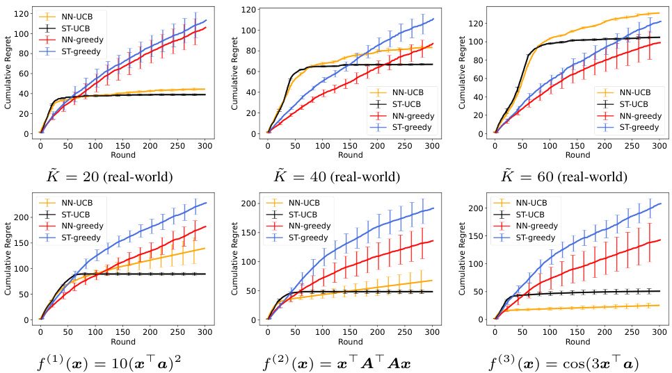
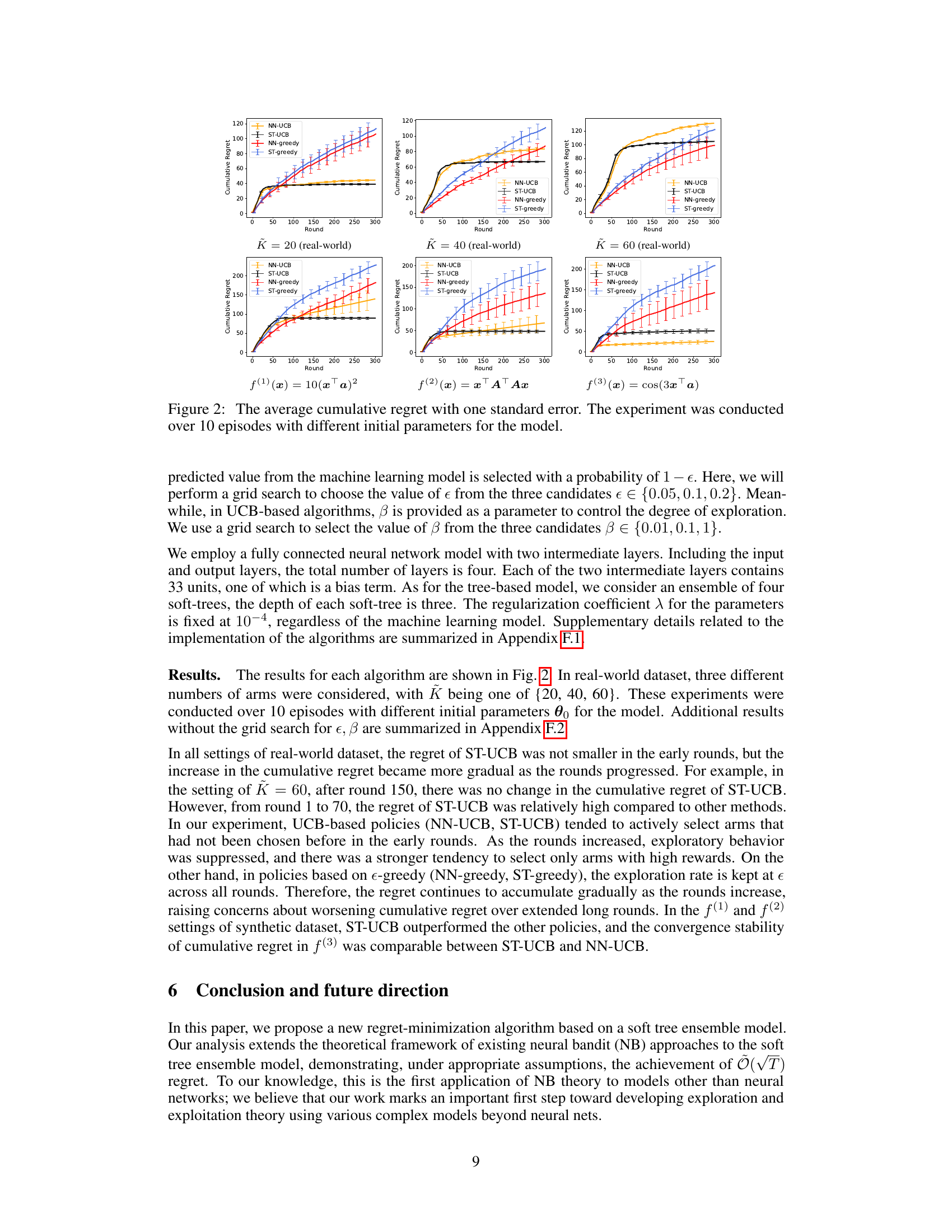
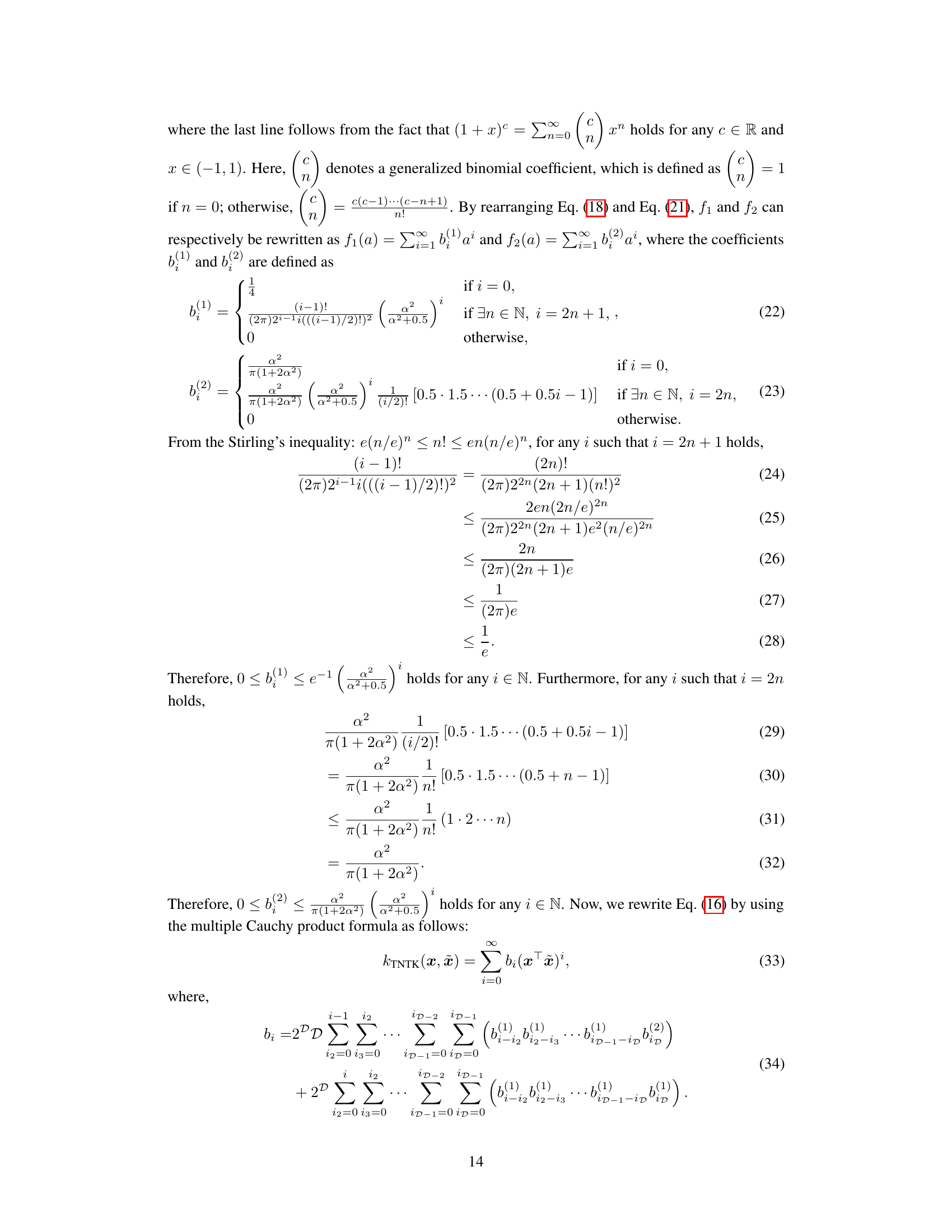
🔼 This figure displays the average cumulative regret across 10 experimental runs for four different bandit algorithms (NN-UCB, ST-UCB, NN-greedy, ST-greedy). Each algorithm’s performance is shown for three different scenarios in the real-world dataset (varying the number of arms K) and three different reward functions in a synthetic dataset. Error bars representing one standard error are included for each data point. The results illustrate the relative performance of the algorithms under different conditions and problem complexities.
read the caption
Figure 2: The average cumulative regret with one standard error. The experiment was conducted over 10 episodes with different initial parameters for the model.
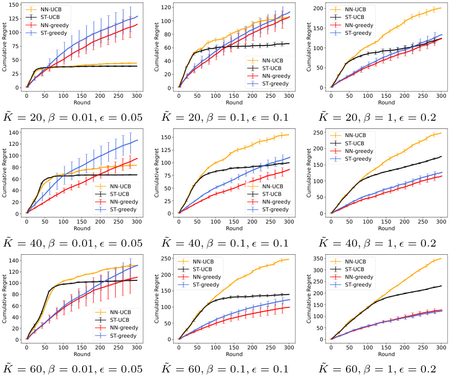
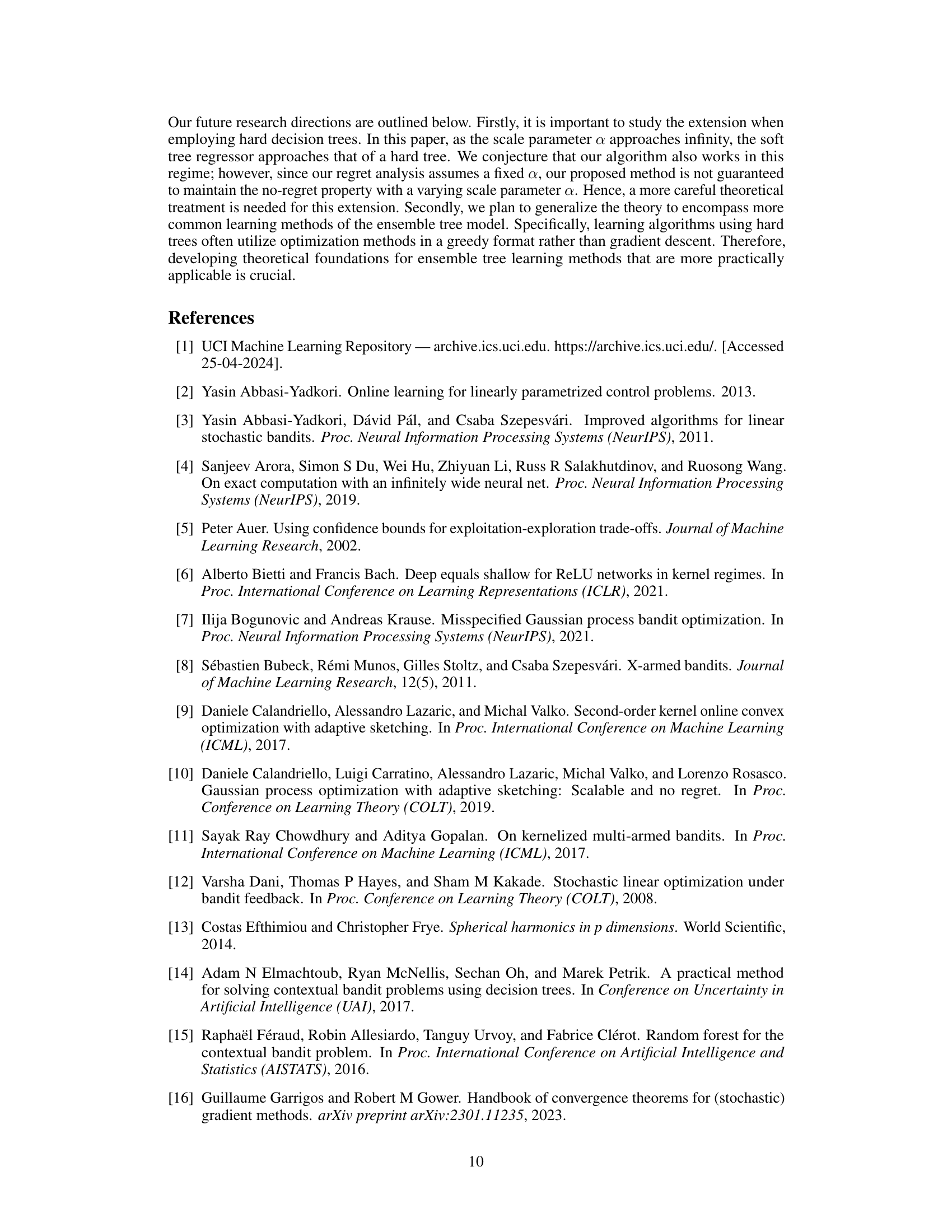
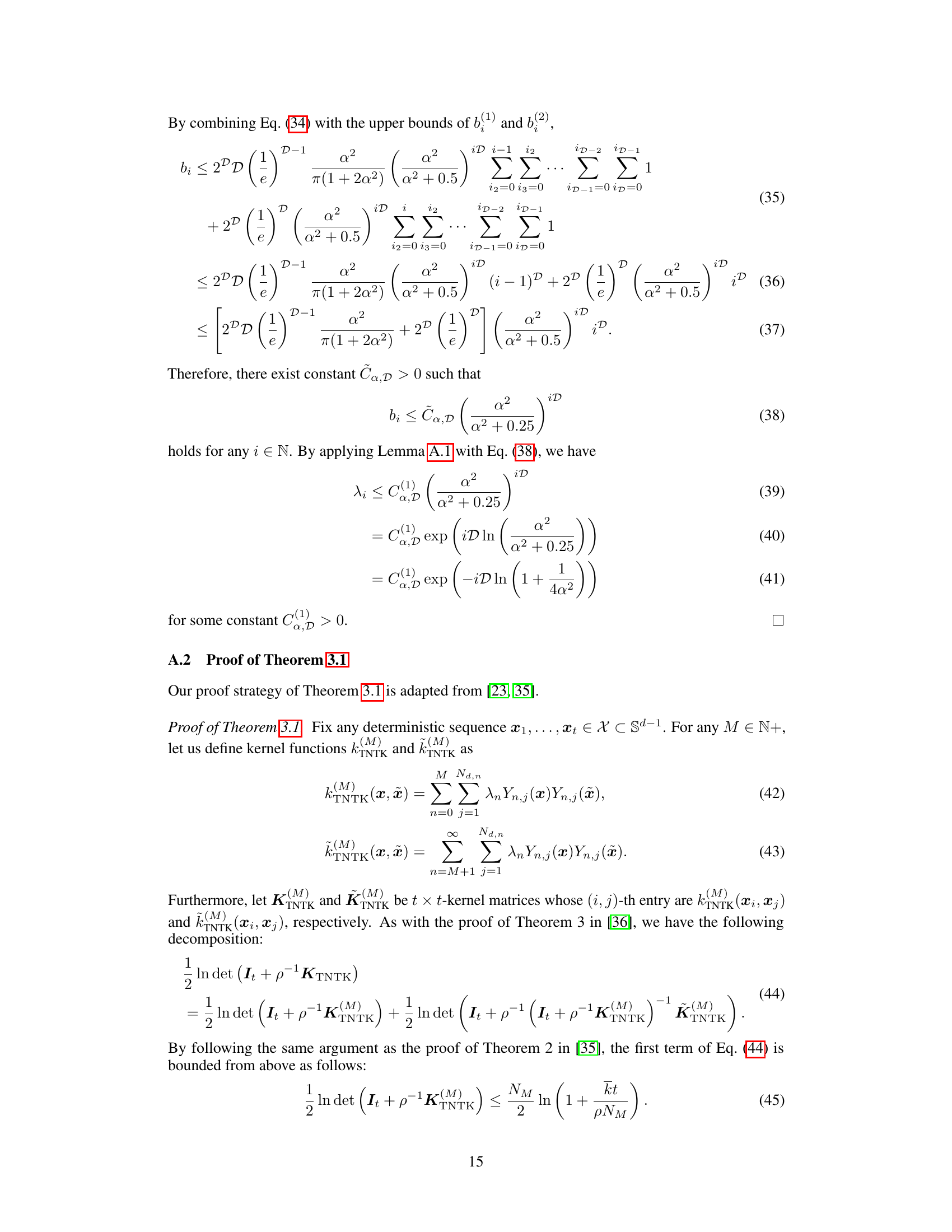
🔼 The figure shows the average cumulative regret across 10 episodes with different initial parameters for three different numbers of arms (K=20, 40, 60) in the real-world dataset. For each number of arms, there are three subplots, each corresponding to a different setting of the exploration parameters (β, ε). The plots compare the performance of four algorithms: NN-UCB, ST-UCB, NN-greedy, and ST-greedy. Error bars representing one standard error are included for each algorithm.
read the caption
Figure 3: The average cumulative regret with one standard error in the real-world dataset.

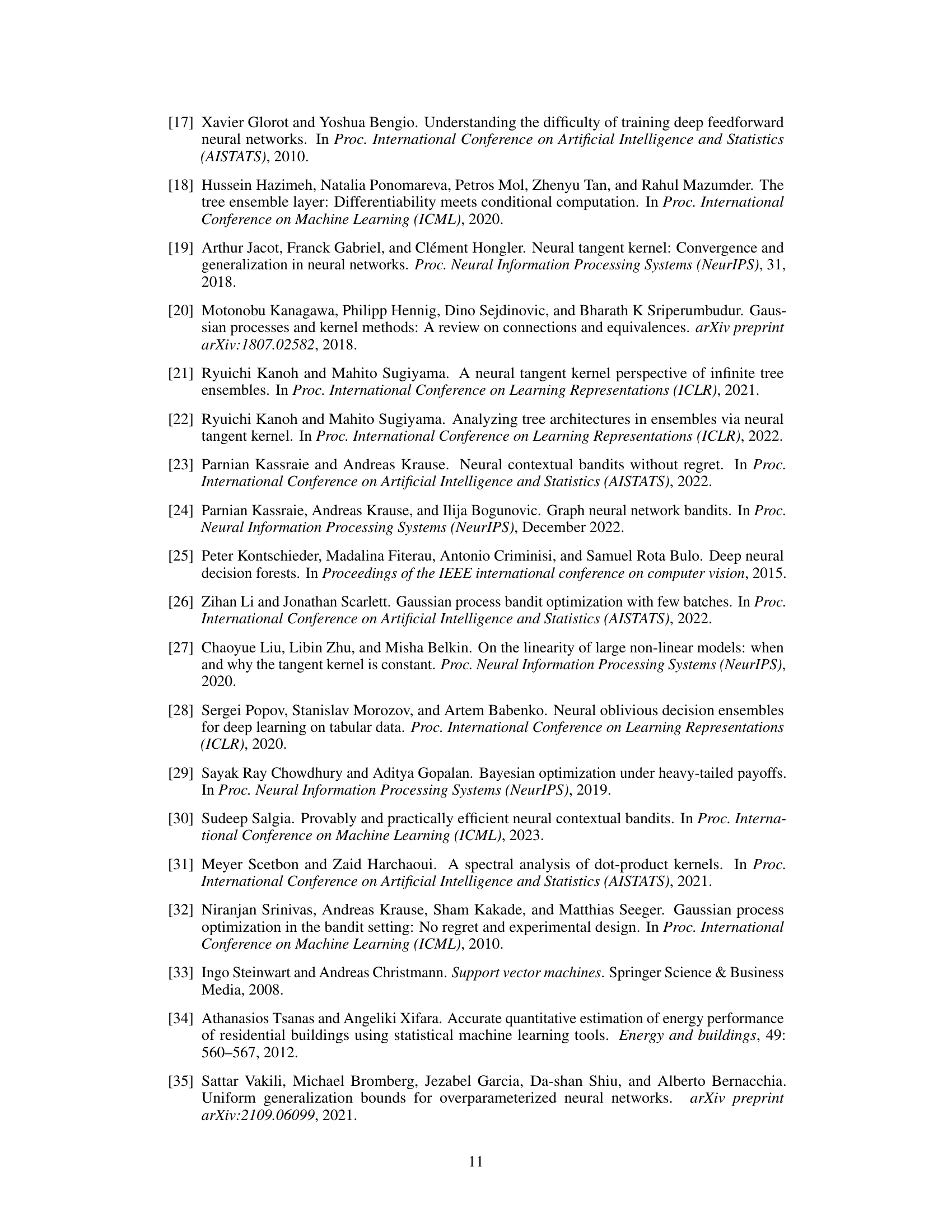
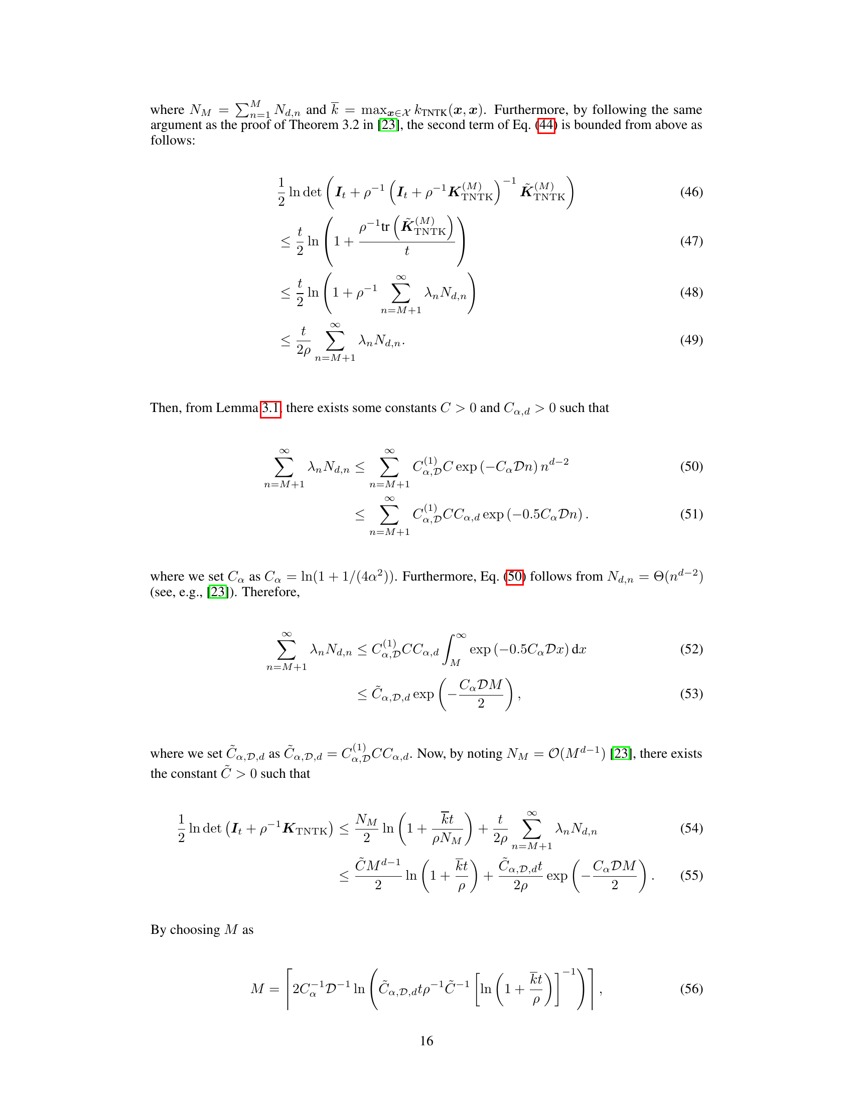
🔼 This figure shows the average cumulative regret of four different bandit algorithms (NN-UCB, ST-UCB, NN-greedy, ST-greedy) across three different synthetic reward functions (f(1), f(2), f(3)) and three different exploration parameters (β = 0.01, 0.1, 1). The error bars represent one standard error. The x-axis represents the number of rounds, and the y-axis represents the cumulative regret.
read the caption
Figure 4: The average cumulative regret with one standard error in the synthetic dataset.
Full paper#

