TL;DR#
Traditional methods for digitizing real-world objects are time-consuming and require significant manual effort. Neural Radiance Fields (NeRFs) offer an automatic approach, but existing NeRF methods often struggle to disentangle lighting from material properties, hindering efficient and realistic scene reconstruction. High-frequency illumination is also challenging to represent accurately in these methods.
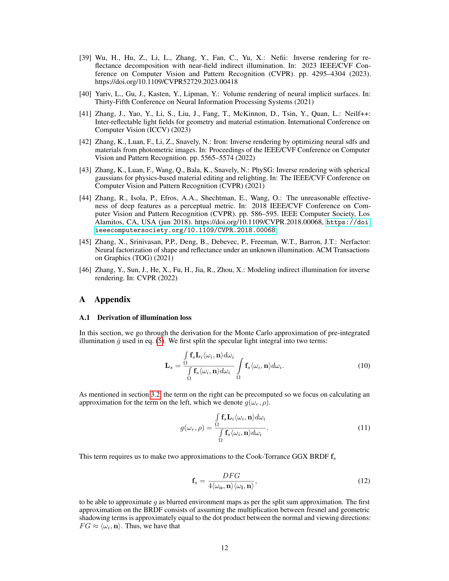
SplitNeRF addresses these limitations by incorporating the split sum approximation, commonly used in real-time image-based lighting, into NeRF pipelines. This approximation splits the rendering equation into two parts: one for pre-integrated illumination and one for material properties. The method models scene lighting with a single scene-specific MLP, accurately representing pre-integrated lighting through a novel regularizer based on efficient Monte Carlo sampling. Additionally, a novel method supervises self-occlusion predictions. Experiments show that SplitNeRF achieves state-of-the-art relighting quality and efficiently estimates scene geometry, material properties, and lighting with under an hour of training on a single NVIDIA A100 GPU.
Key Takeaways#
Why does it matter?#
This paper is important because it presents a novel and efficient method for inverse rendering, a crucial task in computer vision and graphics. The method’s speed and accuracy in estimating scene geometry, lighting, and material properties are significant advancements, opening up new avenues for applications in fields such as digital twin creation, virtual and augmented reality, and 3D modeling. Its efficiency and effectiveness, demonstrated through state-of-the-art results after only 1 hour of training, makes it particularly relevant to current research trends focused on efficient and realistic scene representation.
Visual Insights#
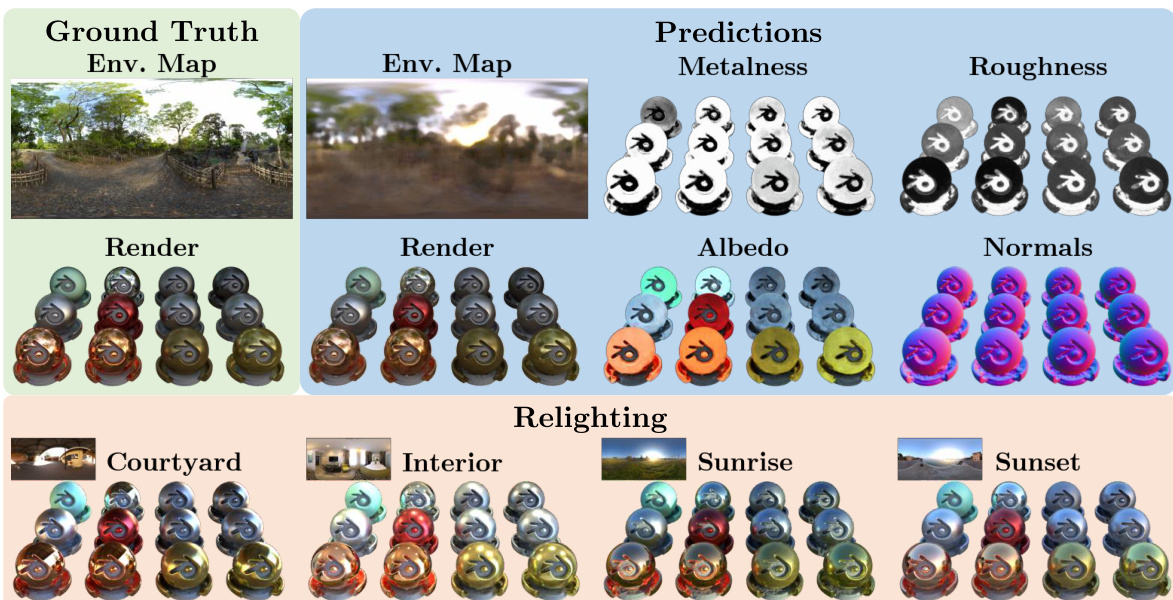
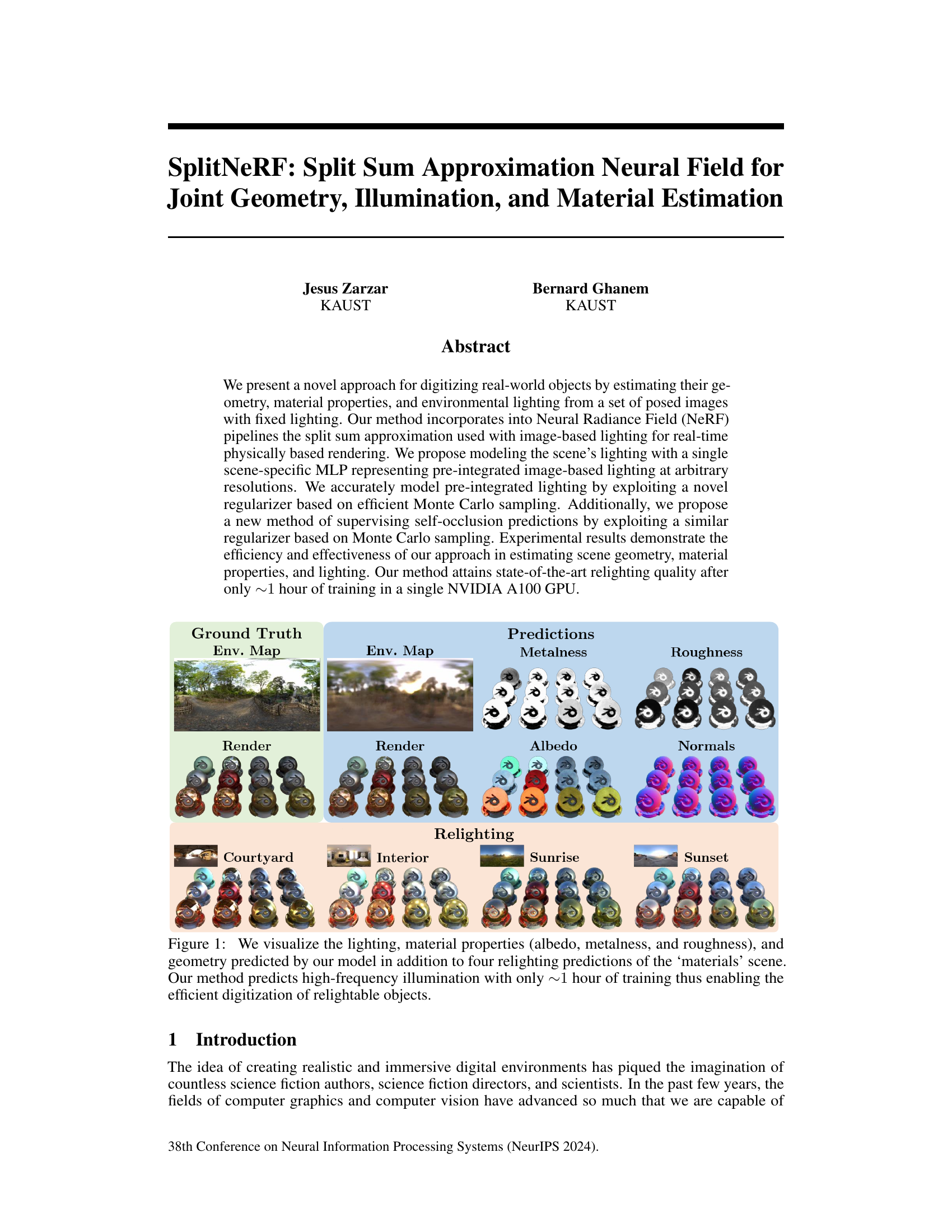
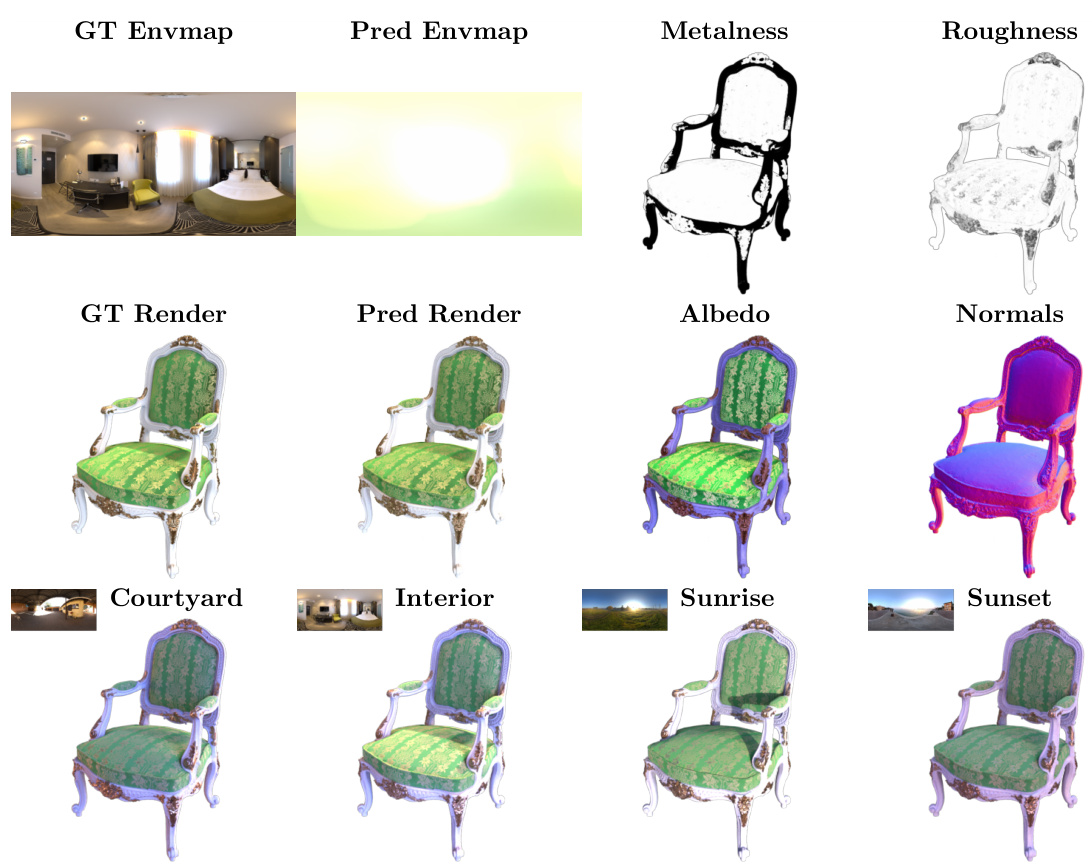
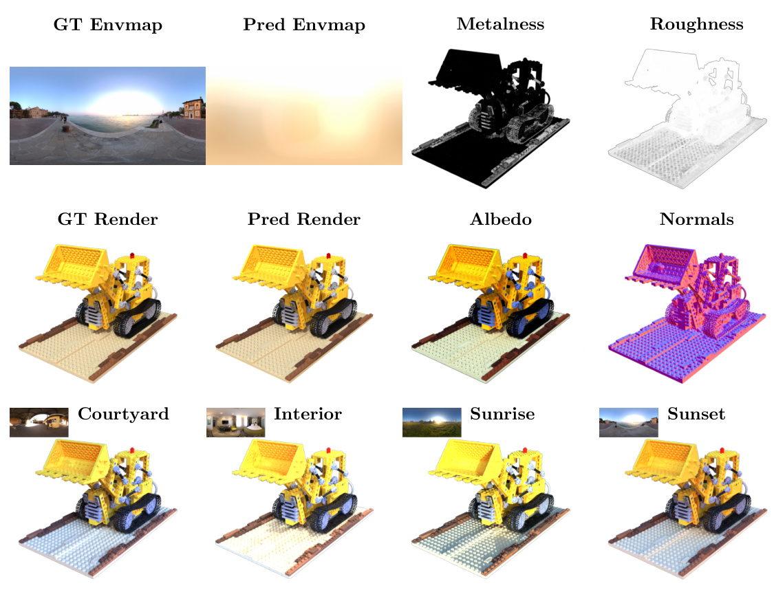
🔼 This figure shows the results of the SplitNeRF model on the ‘materials’ scene. The top row displays the ground truth environment map, a rendered image of the scene, and the model’s predictions for metalness and roughness. The middle row shows the model’s albedo and normal predictions, along with another rendered image. The bottom row demonstrates the model’s ability to relight the scene under four different lighting conditions (‘Courtyard’, ‘Interior’, ‘Sunrise’, ‘Sunset’). The high-quality relighting results, achieved with only one hour of training, highlight the efficiency and effectiveness of the proposed SplitNeRF approach.
read the caption
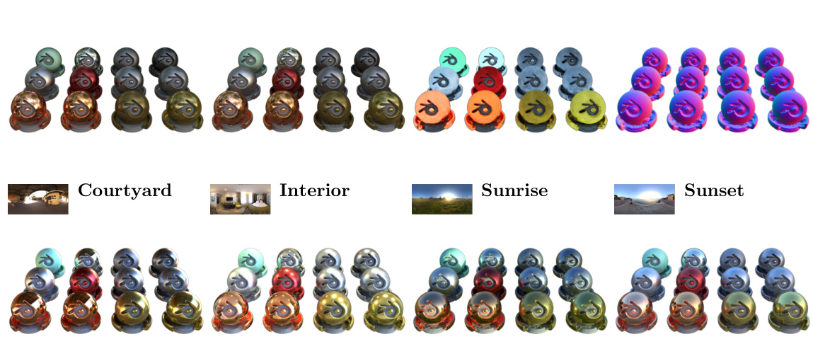
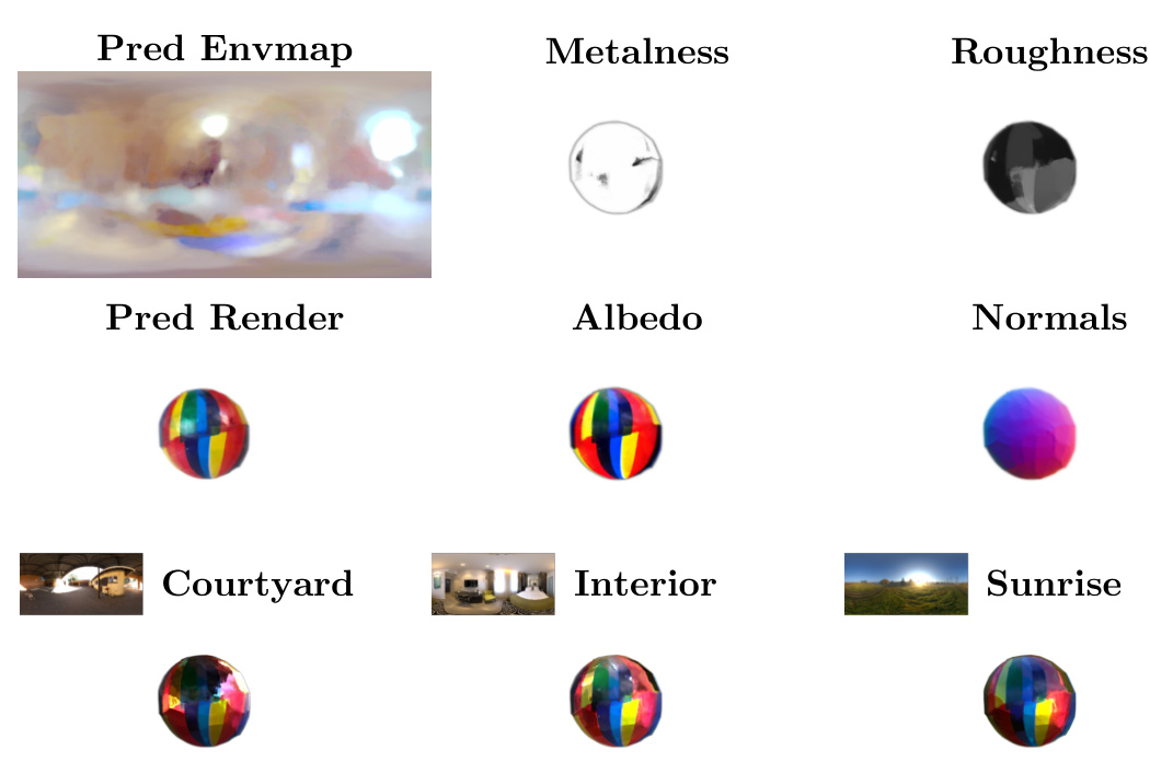
Figure 1: We visualize the lighting, material properties (albedo, metalness, and roughness), and geometry predicted by our model in addition to four relighting predictions of the ‘materials’ scene. Our method predicts high-frequency illumination with only ~1 hour of training thus enabling the efficient digitization of relightable objects.

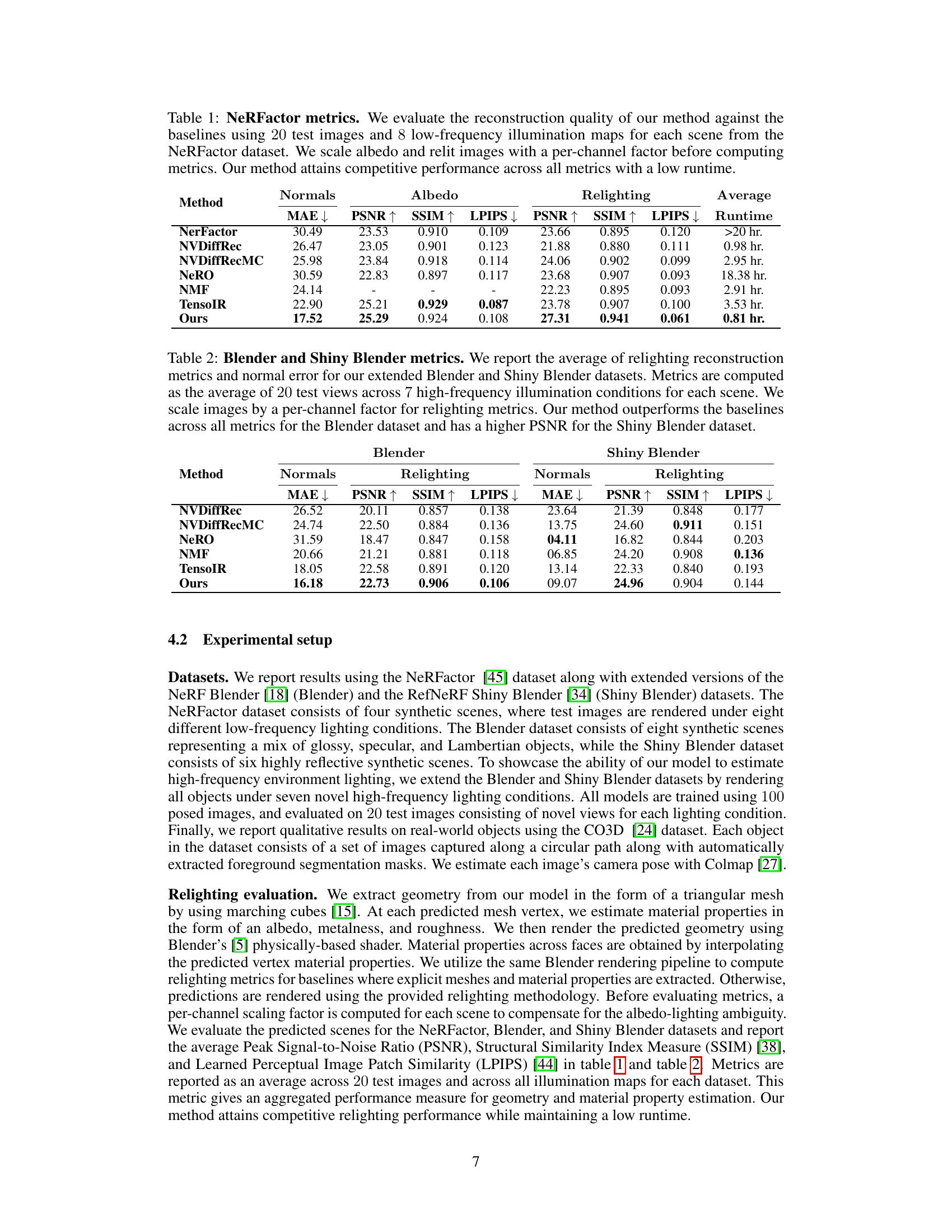
🔼 This table compares the proposed method’s performance against several baselines on the NeRFactor dataset for reconstructing normals, albedo, and relighting. Metrics include MAE, PSNR, SSIM, and LPIPS. The runtime is also reported, highlighting the efficiency of the proposed method.
read the caption
Table 1: NeRFactor metrics. We evaluate the reconstruction quality of our method against the baselines using 20 test images and 8 low-frequency illumination maps for each scene from the NeRFactor dataset. We scale albedo and relit images with a per-channel factor before computing metrics. Our method attains competitive performance across all metrics with a low runtime.
In-depth insights#
Split Sum NeRF#
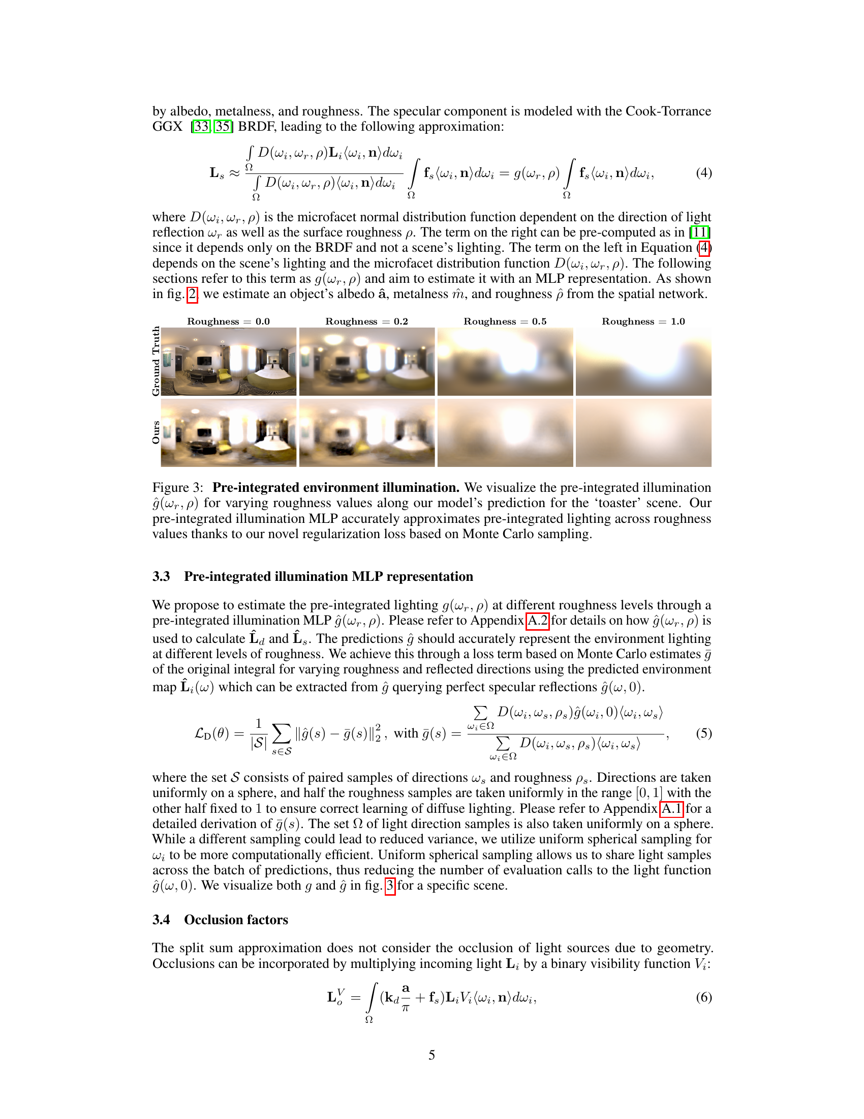
Split Sum NeRF represents a novel approach to neural radiance fields (NeRFs) by integrating the split sum approximation, a technique traditionally used in image-based lighting. This allows for a more efficient and physically accurate modeling of scene illumination by decoupling the material properties from the lighting calculations. The core innovation lies in employing a single MLP to represent pre-integrated lighting, enabling the capture of high-frequency lighting details. This approach is further enhanced by a novel regularizer for precise pre-integrated lighting estimation, leveraging Monte Carlo sampling. Addressing the issue of self-occlusion, often problematic in NeRFs, the method introduces an occlusion factor estimated through a similar Monte Carlo technique, which helps in improving the accuracy of material property predictions. The combined methodology demonstrates a significant improvement in the quality of relighting, material property estimation, and geometry reconstruction, all achieved with considerable computational efficiency as demonstrated by state-of-the-art relighting quality after only an hour of training.
Illumination MLP#
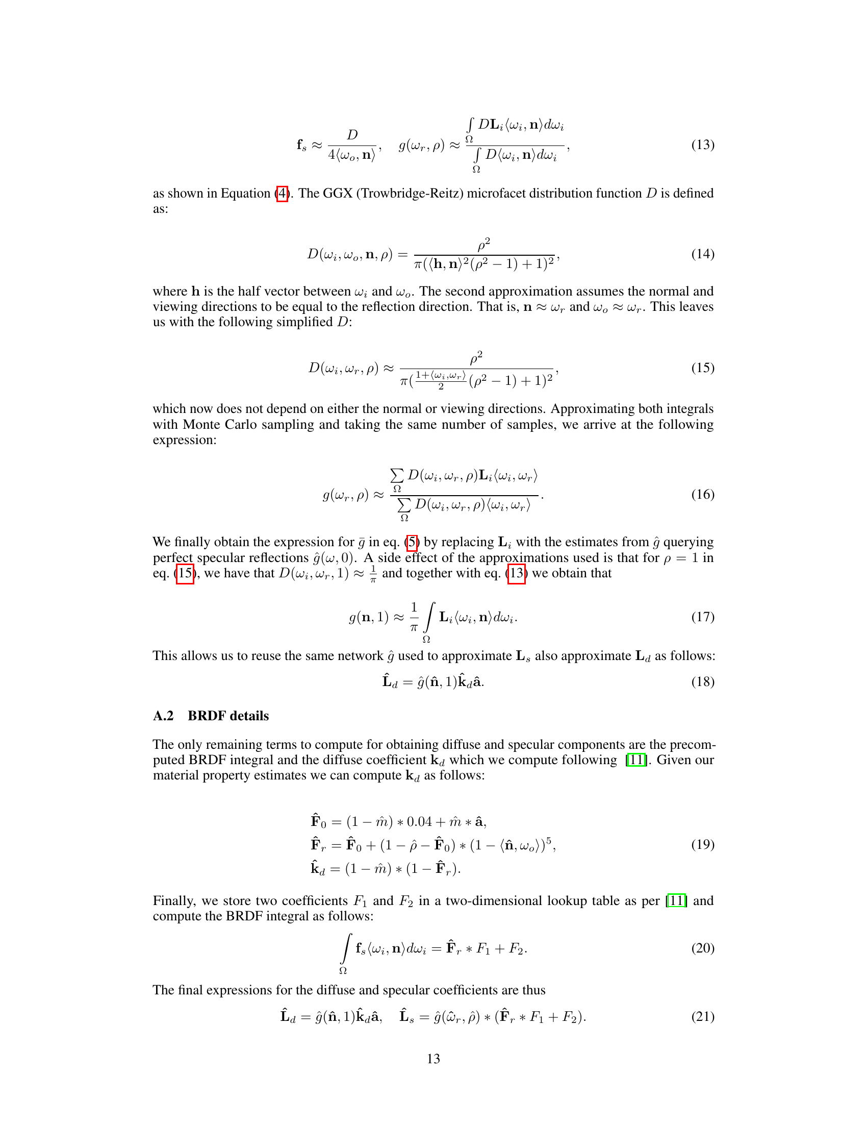
The concept of an “Illumination MLP” in the context of neural radiance fields (NeRFs) for inverse rendering is a clever approach to decoupling scene lighting from material properties. Instead of learning a complex radiance field that entangles both, this method uses a separate Multi-Layer Perceptron (MLP) specifically designed to model pre-integrated lighting. This pre-integration step simplifies the rendering equation, making it more efficient and facilitating high-frequency illumination representation. The MLP’s input typically consists of surface normal and reflection vectors, allowing it to predict the pre-integrated lighting. Supervised training with a novel regularizer based on Monte Carlo sampling further improves accuracy, ensuring the MLP learns a physically meaningful representation. This results in more realistic and high-quality relighting capabilities, outperforming methods where lighting is entangled within scene properties.
Occlusion Factors#
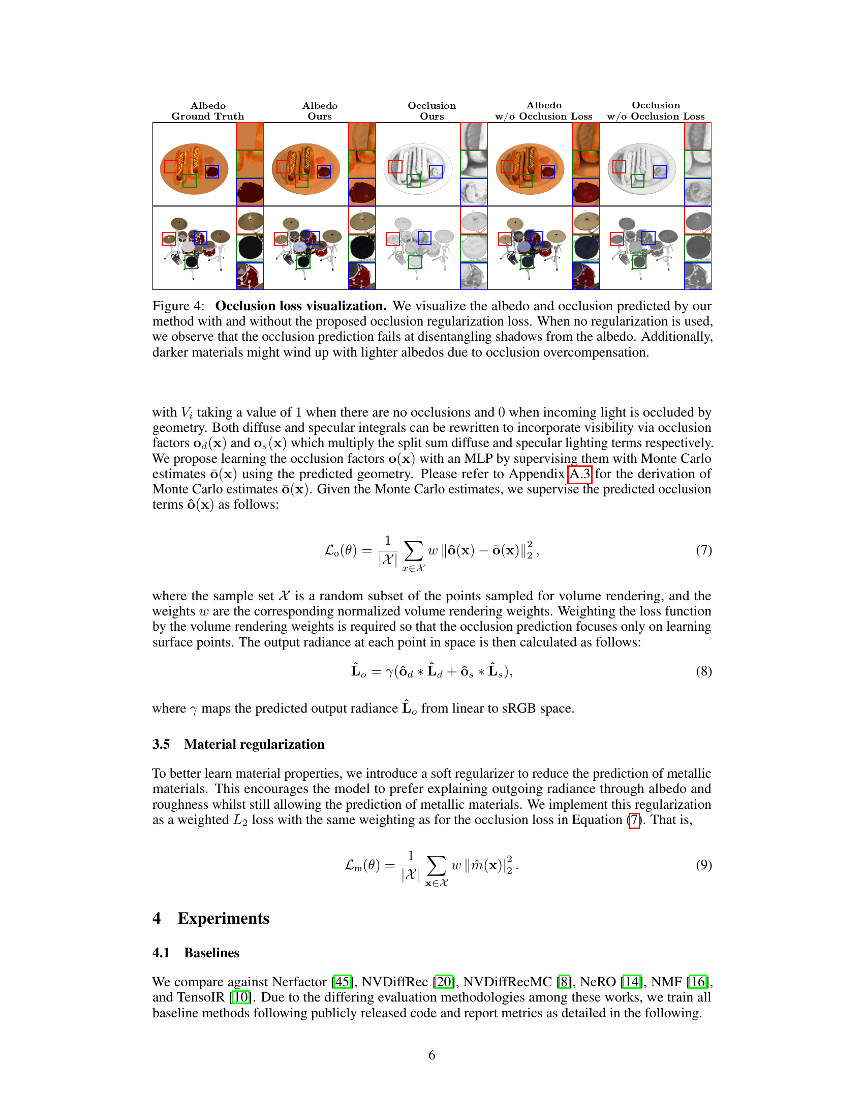
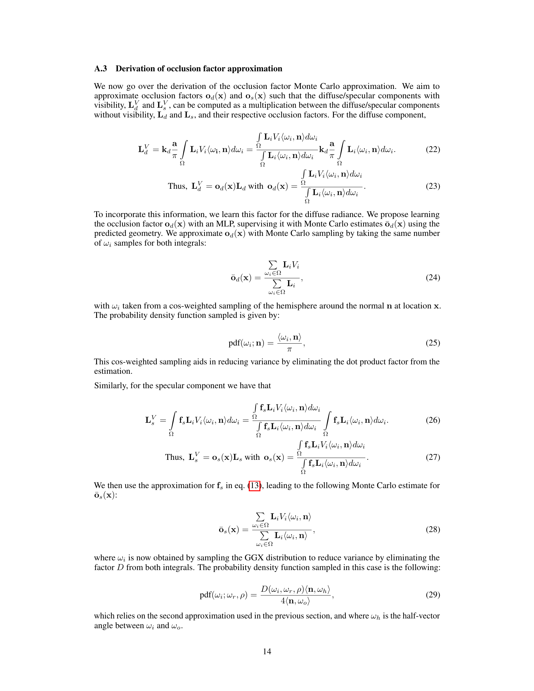
The concept of occlusion factors addresses a critical limitation in traditional rendering techniques, particularly when dealing with complex scenes and indirect lighting. By explicitly modeling the effect of self-occlusion, the accuracy of material property estimation and lighting prediction is significantly improved. The split sum approximation, while efficient, often fails to accurately account for the obscuring effect of geometry on light transport. Occlusion factors act as a multiplicative correction, weighting the incoming light based on whether a given surface point is visible to the light source. This weighting is crucial because shadows are often incorrectly attributed to material properties like albedo, leading to inaccurate rendering. The use of Monte Carlo sampling to estimate occlusion factors demonstrates a sophisticated approach to handle the complex integration problem. This method enables the learning of high-frequency illumination details and enhances the realism of rendered scenes. The introduction of a regularization loss for the occlusion factor ensures accurate learning, thereby further strengthening the overall efficiency and quality of the rendering process.
Material Regularization#
The heading ‘Material Regularization’ suggests a technique to improve the accuracy and realism of material property prediction in a neural rendering model. This is crucial because neural networks often struggle to accurately capture the subtle nuances of real-world materials, leading to artifacts in the rendered images. The regularization likely penalizes unrealistic material properties, such as excessively metallic surfaces, ensuring that the model prioritizes plausible material representations over overly shiny or unrealistic textures. This is achieved by adding a penalty term to the loss function, which discourages the prediction of extreme metallic values. By incorporating such a constraint, the model is less likely to overfit to spurious correlations in the training data and instead learns a more robust representation of material properties that generalizes better to unseen objects. The effectiveness of this approach hinges on the careful selection of the regularization strength and the specific form of the penalty term. Too strong a penalty might suppress physically correct predictions, while too weak a penalty might have little impact on the model’s accuracy. The benefits should include improved albedo prediction, more realistic rendered images, and potentially faster convergence of the training process.
Future of NeRFs#
The future of Neural Radiance Fields (NeRFs) is bright, driven by ongoing research to overcome current limitations. Improving efficiency remains a key focus, enabling real-time rendering and broader applications. Extending NeRF capabilities to handle dynamic scenes, complex materials, and large-scale environments is crucial for wider adoption. Integration with other AI techniques, such as deep learning for scene understanding and object recognition, will unlock more powerful applications. Moreover, hardware acceleration and optimized algorithms will enhance NeRF performance and reduce processing times. Ultimately, NeRFs are poised to revolutionize various fields, from computer graphics and virtual reality to robotics and 3D modeling. Addressing issues like data scarcity, limited generalizability, and the computational cost will be vital for continued progress and widespread adoption.
More visual insights#
More on figures

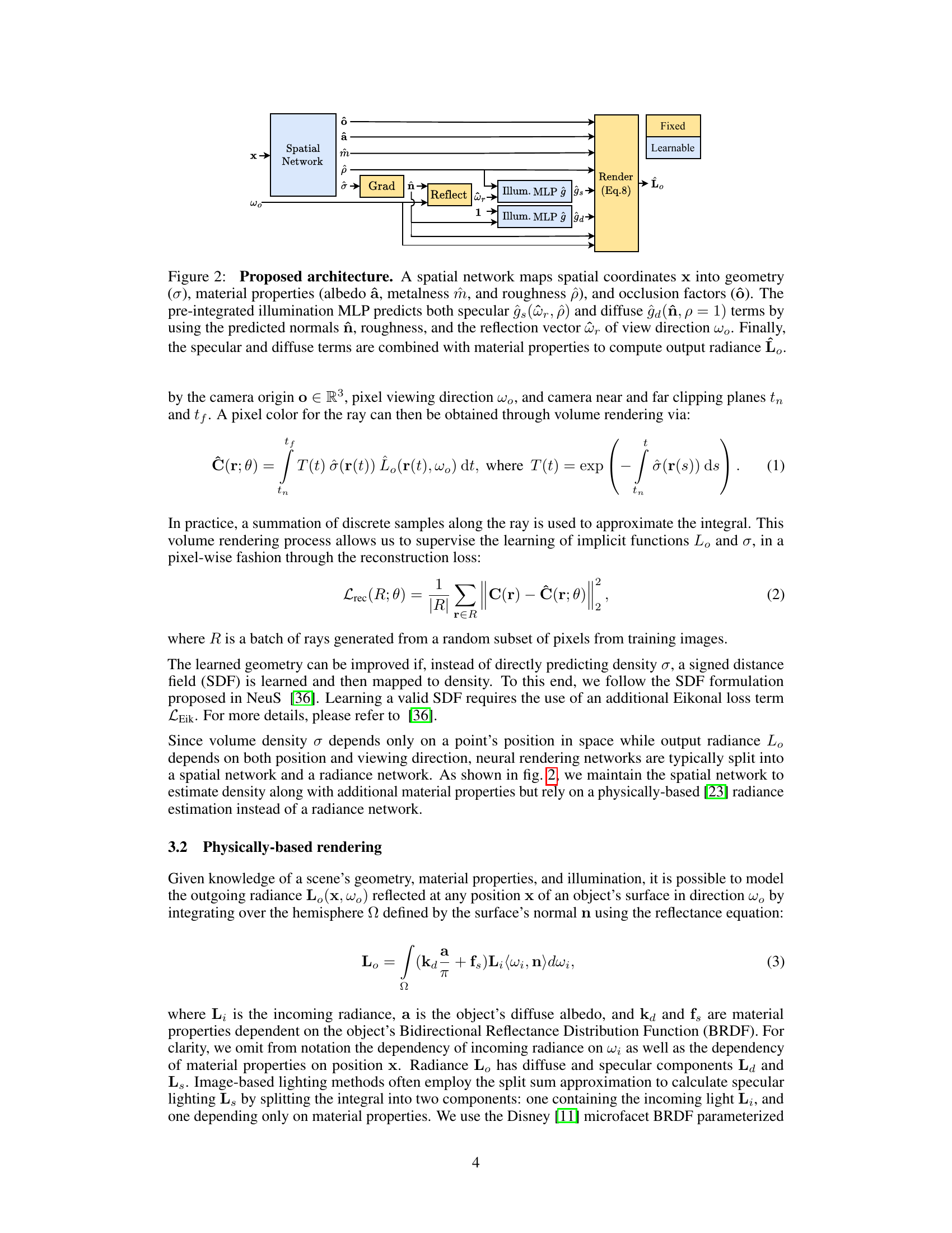
🔼 The figure shows the architecture of the SplitNeRF model. A spatial network takes spatial coordinates as input and outputs geometry, material properties (albedo, metalness, roughness), and occlusion factors. These outputs are then fed into a rendering process. The rendering process also takes in the viewing direction. A pre-integrated illumination MLP takes in the normals, roughness, and reflection vector from the viewing direction and outputs specular and diffuse terms which are combined with the material properties to produce final output radiance.
read the caption
Figure 2: Proposed architecture. A spatial network maps spatial coordinates x into geometry (σ), material properties (albedo â, metalness m, and roughness ô), and occlusion factors (ô). The pre-integrated illumination MLP predicts both specular ĝs (ŵr, p) and diffuse ĝa(ôn, p = 1) terms by using the predicted normals în, roughness, and the reflection vector ŵr of view direction w。. Finally, the specular and diffuse terms are combined with material properties to compute output radiance L。.

🔼 This figure visualizes the pre-integrated illumination predicted by the model for different roughness values on the ’toaster’ scene. It compares the model’s predictions (ours) with the ground truth. The results demonstrate the accuracy of the model’s pre-integrated illumination MLP, which accurately approximates pre-integrated lighting across various roughness levels, thanks to a novel regularization technique based on Monte Carlo sampling.
read the caption
Figure 3: Pre-integrated environment illumination. We visualize the pre-integrated illumination ĝ(ŵr, p) for varying roughness values along our model’s prediction for the ‘toaster’ scene. Our pre-integrated illumination MLP accurately approximates pre-integrated lighting across roughness values thanks to our novel regularization loss based on Monte Carlo sampling.
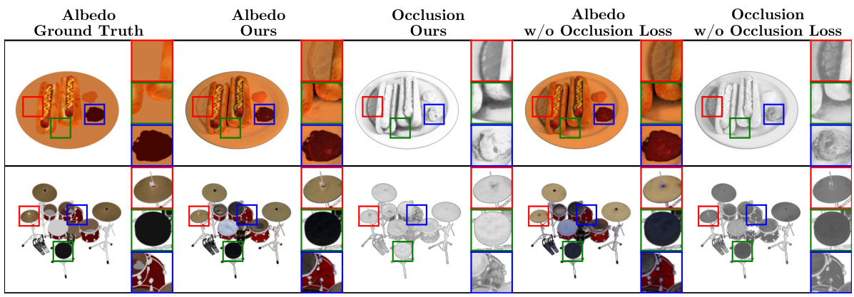
🔼 This figure compares albedo and occlusion predictions with and without the proposed occlusion regularization loss. The left two columns show the results with the loss, demonstrating improved shadow separation and more accurate albedo estimation. The right two columns show the results without the loss, illustrating how shadow misinterpretations lead to inaccurate albedo predictions.
read the caption
Figure 4: Occlusion loss visualization. We visualize the albedo and occlusion predicted by our method with and without the proposed occlusion regularization loss. When no regularization is used, we observe that the occlusion prediction fails at disentangling shadows from the albedo. Additionally, darker materials might wind up with lighter albedos due to occlusion overcompensation.

🔼 This figure shows qualitative results of applying the proposed method to four real-world scenes from the CO3D dataset. Each row represents a different object. The columns show: the ground truth image, a rendering from the proposed model, the predicted albedo (base color), metalness (metallic reflection), roughness (surface texture), normals (surface orientation), and the predicted environment map (lighting conditions). The results demonstrate the model’s ability to accurately reconstruct scene geometry, material properties, and lighting, even in complex real-world scenarios.
read the caption
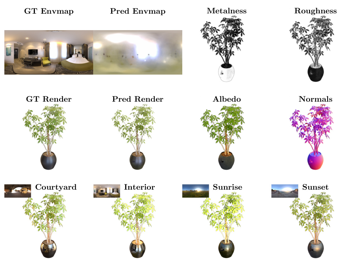
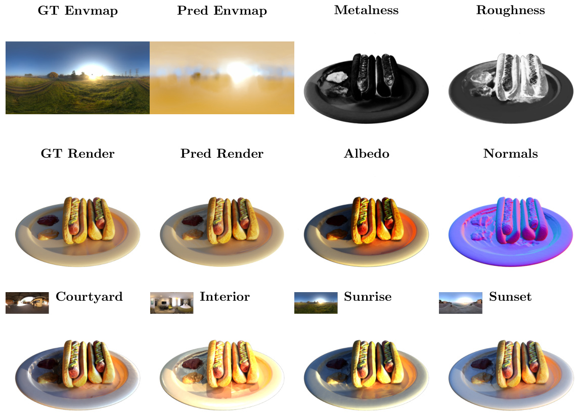
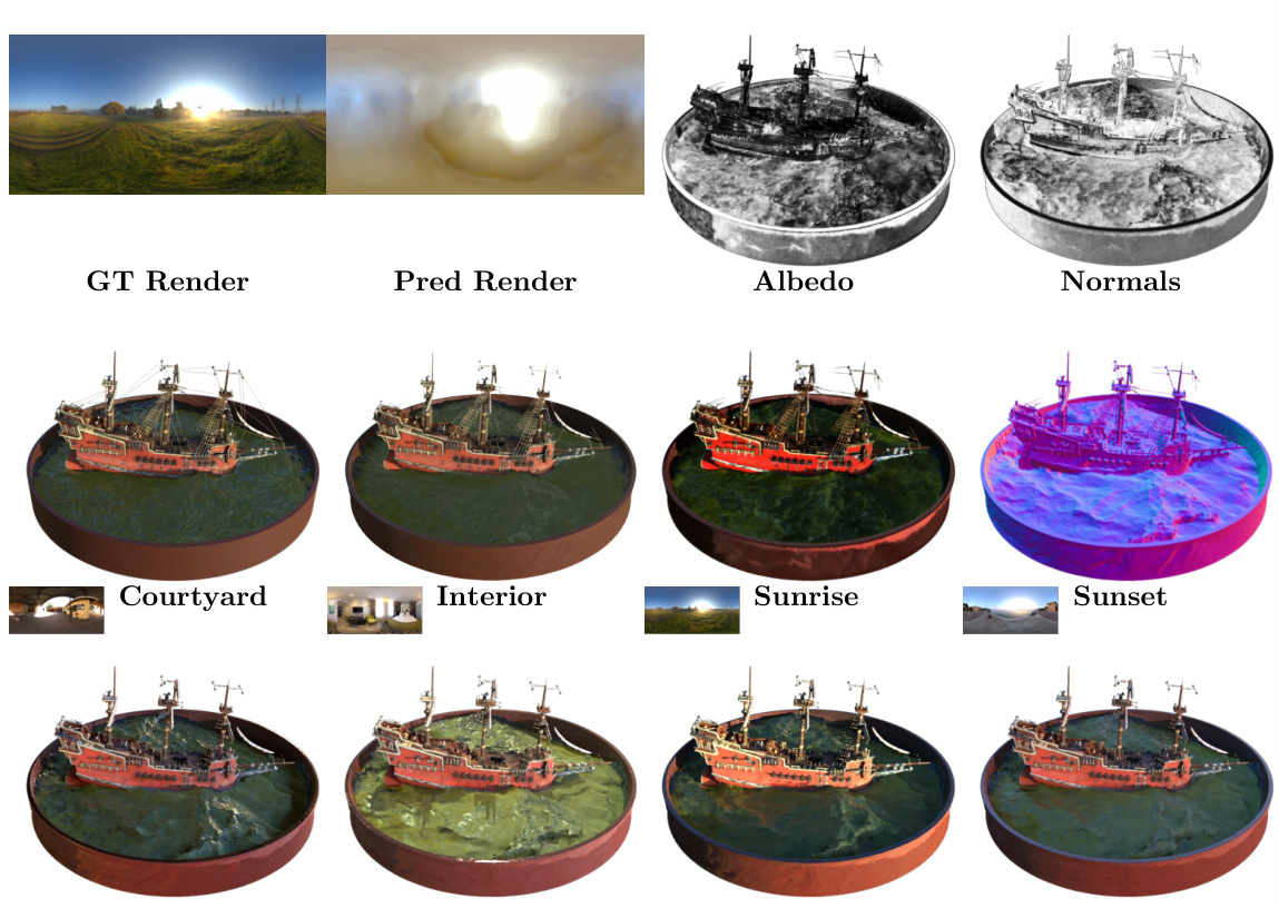
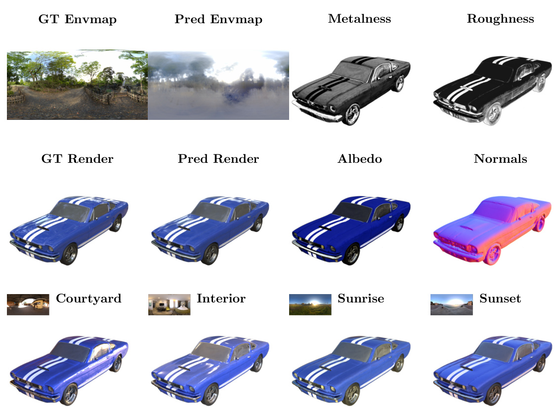
Figure 5: Qualitative real-world results. We present qualitative results on four scenes from the CO3D dataset. Our method can successfully recover object geometry, material properties, and illumination even for challenging scenes captured in the wild.
🔼 This figure shows the results of the proposed method on the ‘materials’ scene. It visualizes the ground truth and predicted lighting environment map, albedo, metalness, roughness, normals, and geometry. Four relighting predictions under different lighting conditions are also shown, demonstrating the model’s ability to predict high-frequency illumination efficiently.
read the caption
Figure 1: We visualize the lighting, material properties (albedo, metalness, and roughness), and geometry predicted by our model in addition to four relighting predictions of the ‘materials’ scene. Our method predicts high-frequency illumination with only ~1 hour of training thus enabling the efficient digitization of relightable objects.
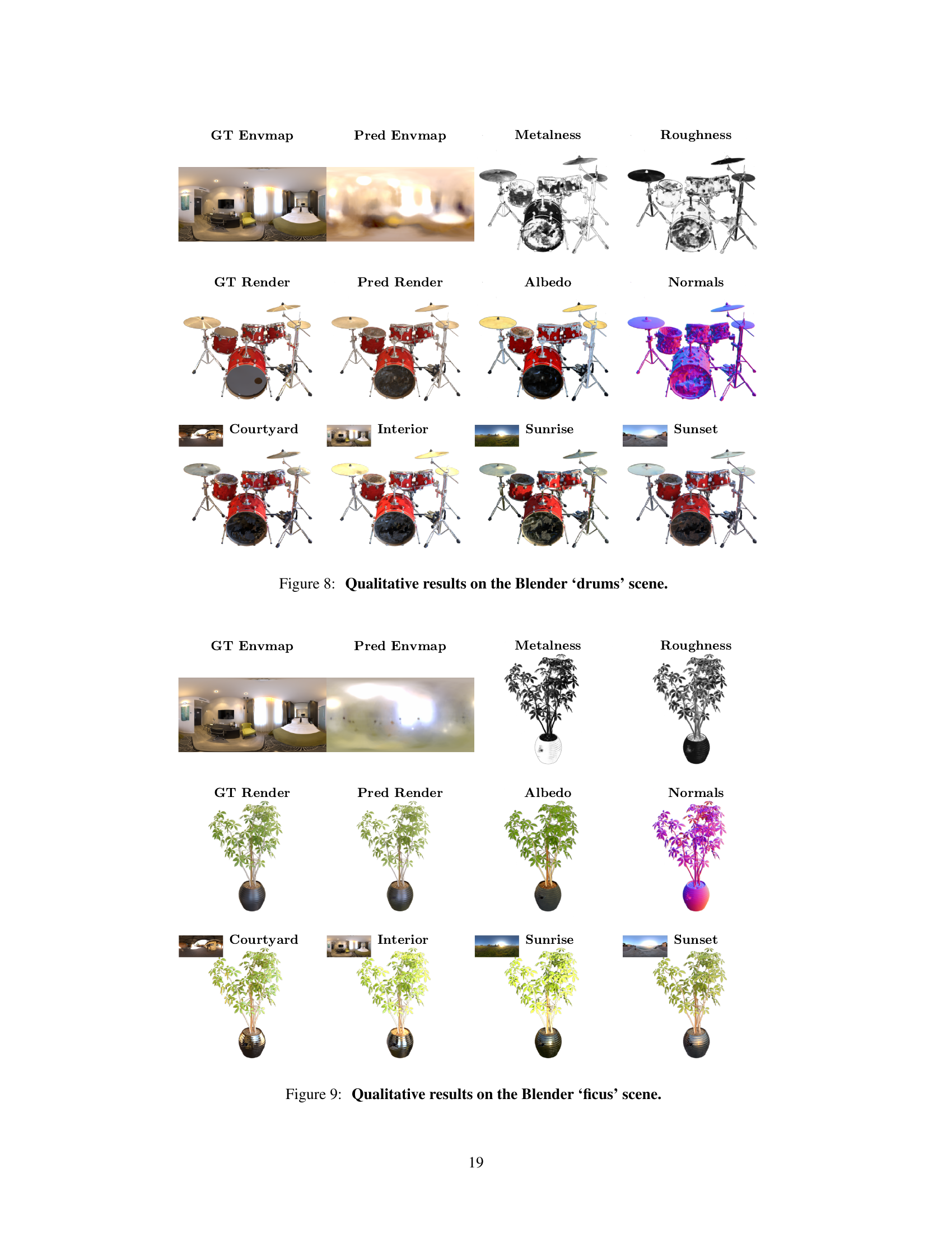
🔼 This figure visualizes the qualitative results of the proposed method on the Blender ‘drums’ scene. It shows the ground truth environment map and the predicted environment map side-by-side, followed by the ground truth and predicted metalness, roughness, albedo, normals, and finally, four relighting results under different lighting conditions: Courtyard, Interior, Sunrise, and Sunset. This demonstrates the model’s ability to accurately estimate scene geometry, material properties, and lighting.
read the caption
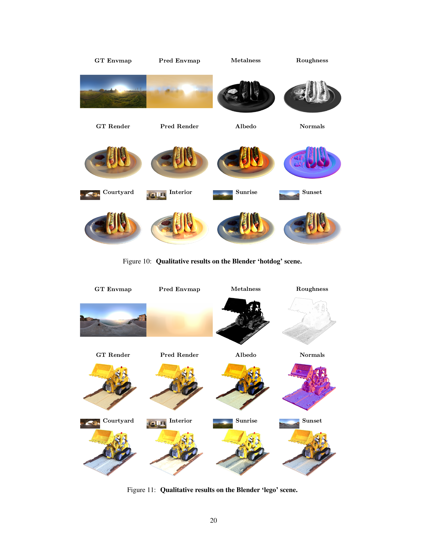
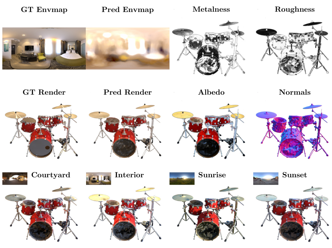
Figure 8: Qualitative results on the Blender ‘drums’ scene.
🔼 This figure shows the results of the SplitNeRF model on the ‘materials’ scene. It displays the ground truth environment map, the predicted environment map, and the model’s predictions for albedo, metalness, roughness, and normals. It also shows four relighting results showcasing how well the model captures and renders lighting conditions.
read the caption
Figure 1: We visualize the lighting, material properties (albedo, metalness, and roughness), and geometry predicted by our model in addition to four relighting predictions of the ‘materials’ scene. Our method predicts high-frequency illumination with only ~1 hour of training thus enabling the efficient digitization of relightable objects.
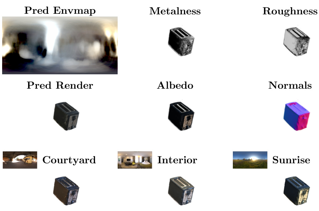
🔼 This figure shows a comparison between the ground truth and the model’s predictions for a scene containing various materials. The top row displays the ground truth environment map, the predicted environment map, and the predicted metalness, and roughness. The middle row displays the ground truth rendering, the predicted rendering, the predicted albedo, and the predicted normals. The bottom row shows the relighting results under four different lighting conditions (Courtyard, Interior, Sunrise, Sunset). The results demonstrate the model’s ability to accurately predict lighting, material properties, and geometry.
read the caption
Figure 1: We visualize the lighting, material properties (albedo, metalness, and roughness), and geometry predicted by our model in addition to four relighting predictions of the ‘materials’ scene. Our method predicts high-frequency illumination with only ~1 hour of training thus enabling the efficient digitization of relightable objects.
🔼 This figure shows qualitative results of applying the proposed method to four real-world scenes from the CO3D dataset. The results demonstrate the ability of the method to accurately estimate the scene’s geometry, material properties (albedo, metalness, roughness, normals), and environmental lighting, even in complex real-world scenarios with challenging lighting and occlusion conditions.
read the caption
Figure 5: Qualitative real-world results. We present qualitative results on four scenes from the CO3D dataset. Our method can successfully recover object geometry, material properties, and illumination even for challenging scenes captured in the wild.

🔼 The figure shows the results of the proposed method on a scene containing various materials. The ground truth environment map and renderings are displayed alongside the model’s predictions for lighting, material properties (albedo, metalness, and roughness), geometry, and four relighting predictions under different lighting conditions. The results demonstrate the method’s ability to predict high-frequency illumination and accurately reconstruct the scene’s geometry and material properties.
read the caption
Figure 1: We visualize the lighting, material properties (albedo, metalness, and roughness), and geometry predicted by our model in addition to four relighting predictions of the ‘materials’ scene. Our method predicts high-frequency illumination with only ~1 hour of training thus enabling the efficient digitization of relightable objects.
🔼 This figure shows the results of applying the SplitNeRF model to a scene containing various materials. The top row displays the ground truth environment map and renderings of the scene. The second row displays the predictions made by SplitNeRF, including albedo, metalness, roughness, normals, and the environment map. The bottom row shows four different relighting predictions generated using the estimated lighting and material properties. The figure highlights the model’s ability to accurately predict high-frequency illumination and material properties with a relatively short training time, enabling efficient digitization of relightable objects.
read the caption
Figure 1: We visualize the lighting, material properties (albedo, metalness, and roughness), and geometry predicted by our model in addition to four relighting predictions of the ‘materials’ scene. Our method predicts high-frequency illumination with only ~1 hour of training thus enabling the efficient digitization of relightable objects.

🔼 This figure visualizes the results of the SplitNeRF model on the ‘materials’ scene. It shows the ground truth environment map, predicted environment map, predicted albedo, metalness, roughness, normals, and four relighting results (courtyard, interior, sunrise, and sunset). The figure highlights the model’s ability to predict high-frequency lighting details with just one hour of training, demonstrating efficient digitization of objects suitable for relighting.
read the caption
Figure 1: We visualize the lighting, material properties (albedo, metalness, and roughness), and geometry predicted by our model in addition to four relighting predictions of the ‘materials’ scene. Our method predicts high-frequency illumination with only ~1 hour of training thus enabling the efficient digitization of relightable objects.
🔼 This figure shows the results of the SplitNeRF model on the ‘materials’ scene. It displays the ground truth environment map and render, alongside the model’s predictions for the environment map, albedo, metalness, roughness, normals, and four relighting variations (Courtyard, Interior, Sunrise, Sunset). The high-frequency details in the illumination highlight the efficiency of the model, which achieves these results with only about one hour of training.
read the caption
Figure 1: We visualize the lighting, material properties (albedo, metalness, and roughness), and geometry predicted by our model in addition to four relighting predictions of the ‘materials’ scene. Our method predicts high-frequency illumination with only ~1 hour of training thus enabling the efficient digitization of relightable objects.
🔼 This figure shows the results of the proposed method on the ‘materials’ scene. It visualizes the predicted lighting, albedo, metalness, roughness, normals, and geometry. Four different relighting scenarios are also presented, demonstrating the model’s ability to accurately predict high-frequency illumination with just one hour of training.
read the caption
Figure 1: We visualize the lighting, material properties (albedo, metalness, and roughness), and geometry predicted by our model in addition to four relighting predictions of the ‘materials’ scene. Our method predicts high-frequency illumination with only ~1 hour of training thus enabling the efficient digitization of relightable objects.
🔼 This figure shows a comparison between the ground truth and the model’s predictions for various aspects of a 3D scene, including lighting, material properties (albedo, metalness, roughness), and geometry. The model’s predictions are shown alongside four different relighting conditions, demonstrating the model’s ability to accurately capture high-frequency illumination details with minimal training time.
read the caption
Figure 1: We visualize the lighting, material properties (albedo, metalness, and roughness), and geometry predicted by our model in addition to four relighting predictions of the ‘materials’ scene. Our method predicts high-frequency illumination with only ~1 hour of training thus enabling the efficient digitization of relightable objects.
🔼 This figure shows the results of the proposed method on the ‘materials’ scene. It visualizes the ground truth and predicted lighting, albedo, metalness, roughness, normals, and geometry. Four different relighting scenarios are also shown to highlight the ability of the model to accurately predict high-frequency illumination from a single hour of training. The scene is composed of several differently colored and textured spheres.
read the caption
Figure 1: We visualize the lighting, material properties (albedo, metalness, and roughness), and geometry predicted by our model in addition to four relighting predictions of the ‘materials’ scene. Our method predicts high-frequency illumination with only ~1 hour of training thus enabling the efficient digitization of relightable objects.
🔼 This figure shows a comparison between the ground truth and the model’s predictions for a scene containing various materials. It demonstrates the model’s ability to accurately predict lighting, material properties (albedo, metalness, and roughness), and geometry. The four relighting predictions showcase the model’s capacity for generating realistic renderings under different lighting conditions.
read the caption
Figure 1: We visualize the lighting, material properties (albedo, metalness, and roughness), and geometry predicted by our model in addition to four relighting predictions of the ‘materials’ scene. Our method predicts high-frequency illumination with only ~1 hour of training thus enabling the efficient digitization of relightable objects.
🔼 This figure visualizes the results of the proposed method on the ‘materials’ scene. It shows the ground truth environment map, the predicted environment map, the predicted material properties (albedo, metalness, and roughness), the predicted normals, and four relighting predictions under different lighting conditions. The results demonstrate the method’s ability to accurately predict high-frequency illumination and material properties with only a short training time.
read the caption
Figure 1: We visualize the lighting, material properties (albedo, metalness, and roughness), and geometry predicted by our model in addition to four relighting predictions of the ‘materials’ scene. Our method predicts high-frequency illumination with only ~1 hour of training thus enabling the efficient digitization of relightable objects.

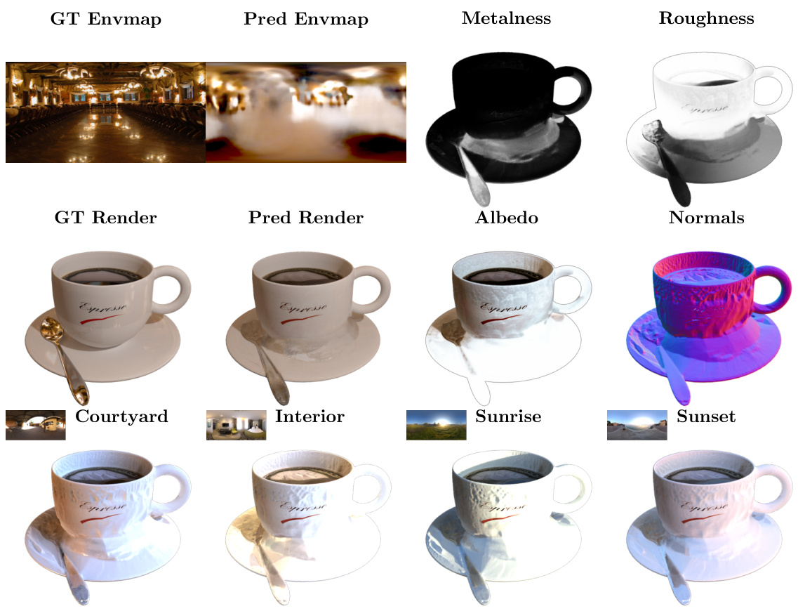
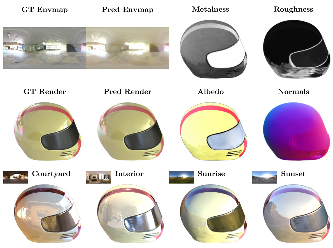
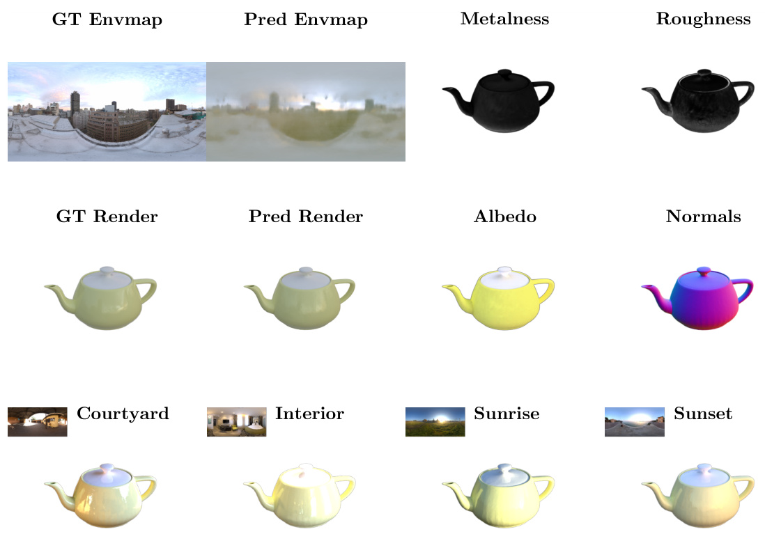
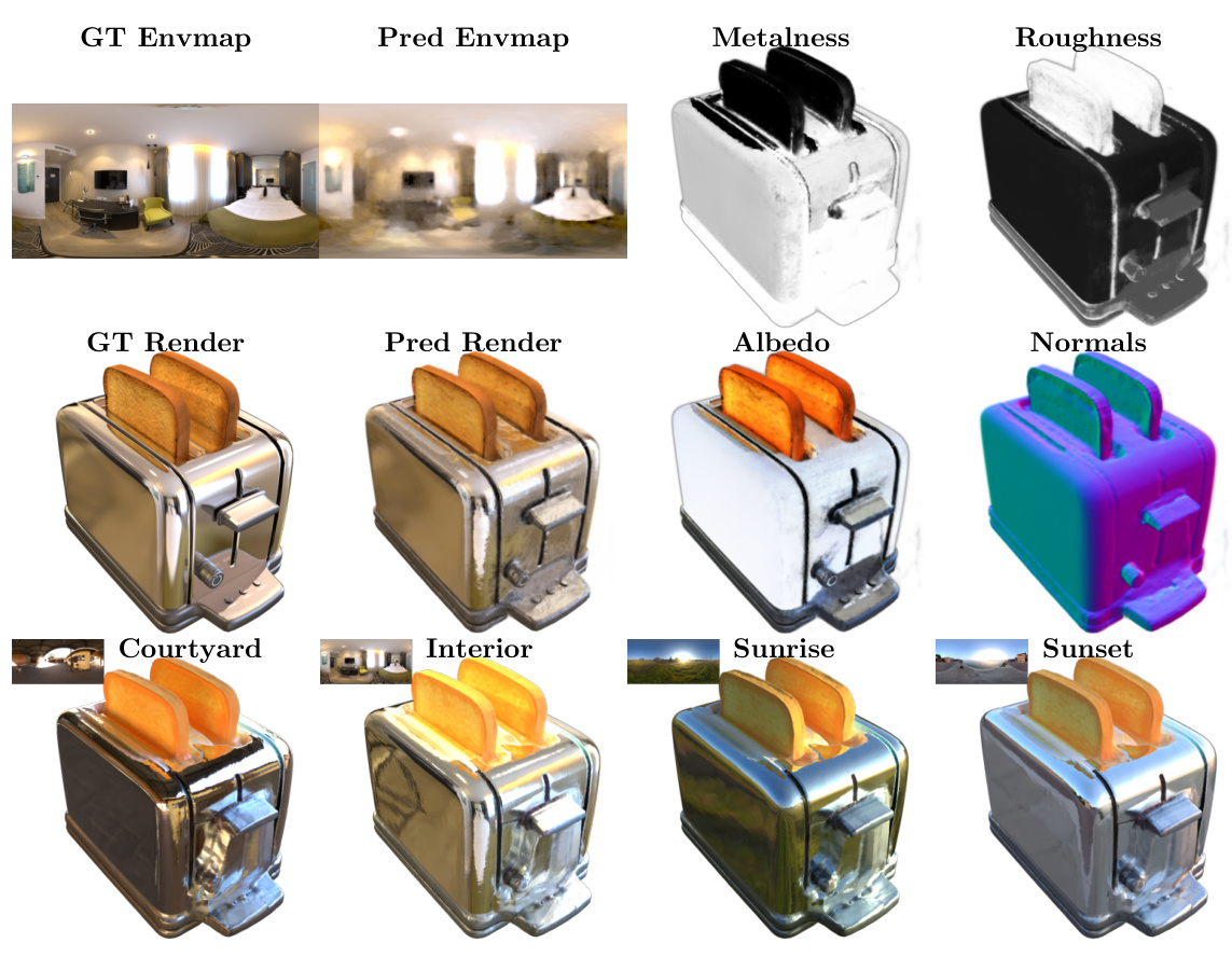
🔼 This figure shows qualitative results of applying the SplitNeRF model to four real-world scenes from the CO3D dataset. For each scene, it displays the ground truth environment map, the model’s predicted environment map, and the predicted metalness, roughness, albedo, normals, and four relighting results under different lighting conditions (‘Courtyard’, ‘Interior’, ‘Sunrise’, ‘Sunset’). The results demonstrate that the model can effectively reconstruct object geometry, material properties, and lighting, even in complex, real-world settings.
read the caption
Figure 5: Qualitative real-world results. We present qualitative results on four scenes from the CO3D dataset. Our method can successfully recover object geometry, material properties, and illumination even for challenging scenes captured in the wild.
🔼 This figure shows the results of the proposed method on the ‘materials’ scene. It visualizes the ground truth and predicted environment map, albedo, metalness, roughness, normals, and geometry. Four relighting scenarios are also shown, demonstrating the model’s ability to accurately capture high-frequency illumination details with only an hour of training.
read the caption
Figure 1: We visualize the lighting, material properties (albedo, metalness, and roughness), and geometry predicted by our model in addition to four relighting predictions of the ‘materials’ scene. Our method predicts high-frequency illumination with only ~1 hour of training thus enabling the efficient digitization of relightable objects.
🔼 This figure showcases the model’s performance on real-world objects from the CO3D dataset. It demonstrates the model’s ability to accurately predict the environment map, object albedo, metalness, roughness, normals, and geometry. Four different relighting scenarios are presented (‘Courtyard’, ‘Interior’, ‘Sunrise’, ‘Sunset’) to highlight the robustness of the predicted lighting and material properties.
read the caption
Figure 5: Qualitative real-world results. We present qualitative results on four scenes from the CO3D dataset. Our method can successfully recover object geometry, material properties, and illumination even for challenging scenes captured in the wild.

🔼 This figure shows the results of the SplitNeRF model on the ‘materials’ scene. It displays the ground truth environment map, the environment map predicted by the model, and the predicted material properties (albedo, metalness, roughness) and geometry. Four additional images showcase the model’s ability to relight the scene with different lighting conditions (Courtyard, Interior, Sunrise, Sunset). The high-frequency detail in the lighting and the speed at which the model achieves this are highlighted.
read the caption
Figure 1: We visualize the lighting, material properties (albedo, metalness, and roughness), and geometry predicted by our model in addition to four relighting predictions of the ‘materials’ scene. Our method predicts high-frequency illumination with only ~1 hour of training thus enabling the efficient digitization of relightable objects.
More on tables

🔼 This table compares the proposed method against baselines on two datasets: Blender and Shiny Blender. The evaluation metrics include Mean Absolute Error (MAE) for normals, Peak Signal-to-Noise Ratio (PSNR) and Structural Similarity Index Measure (SSIM) for relighting and albedo, and Learned Perceptual Image Patch Similarity (LPIPS) for relighting. The results show that the proposed method achieves superior performance compared to existing state-of-the-art methods across all metrics on the Blender dataset and has better PSNR than the baselines on the Shiny Blender dataset. The experiments included high-frequency illumination conditions for a more rigorous evaluation.
read the caption
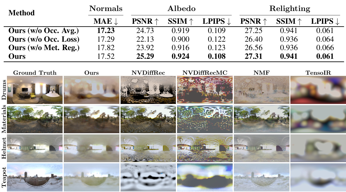
Table 2: Blender and Shiny Blender metrics. We report the average of relighting reconstruction metrics and normal error for our extended Blender and Shiny Blender datasets. Metrics are computed as the average of 20 test views across 7 high-frequency illumination conditions for each scene. We scale images by a per-channel factor for relighting metrics. Our method outperforms the baselines across all metrics for the Blender dataset and has a higher PSNR for the Shiny Blender dataset.
🔼 This table presents a quantitative comparison of the proposed method against several baselines on the NeRFactor dataset. Metrics for normals, albedo, and relighting are shown, along with the runtime. The results demonstrate that the proposed method achieves competitive performance across all metrics while being significantly faster than most baselines.
read the caption
Table 1: NeRFactor metrics. We evaluate the reconstruction quality of our method against the baselines using 20 test images and 8 low-frequency illumination maps for each scene from the NeRFactor dataset. We scale albedo and relit images with a per-channel factor before computing metrics. Our method attains competitive performance across all metrics with a low runtime.

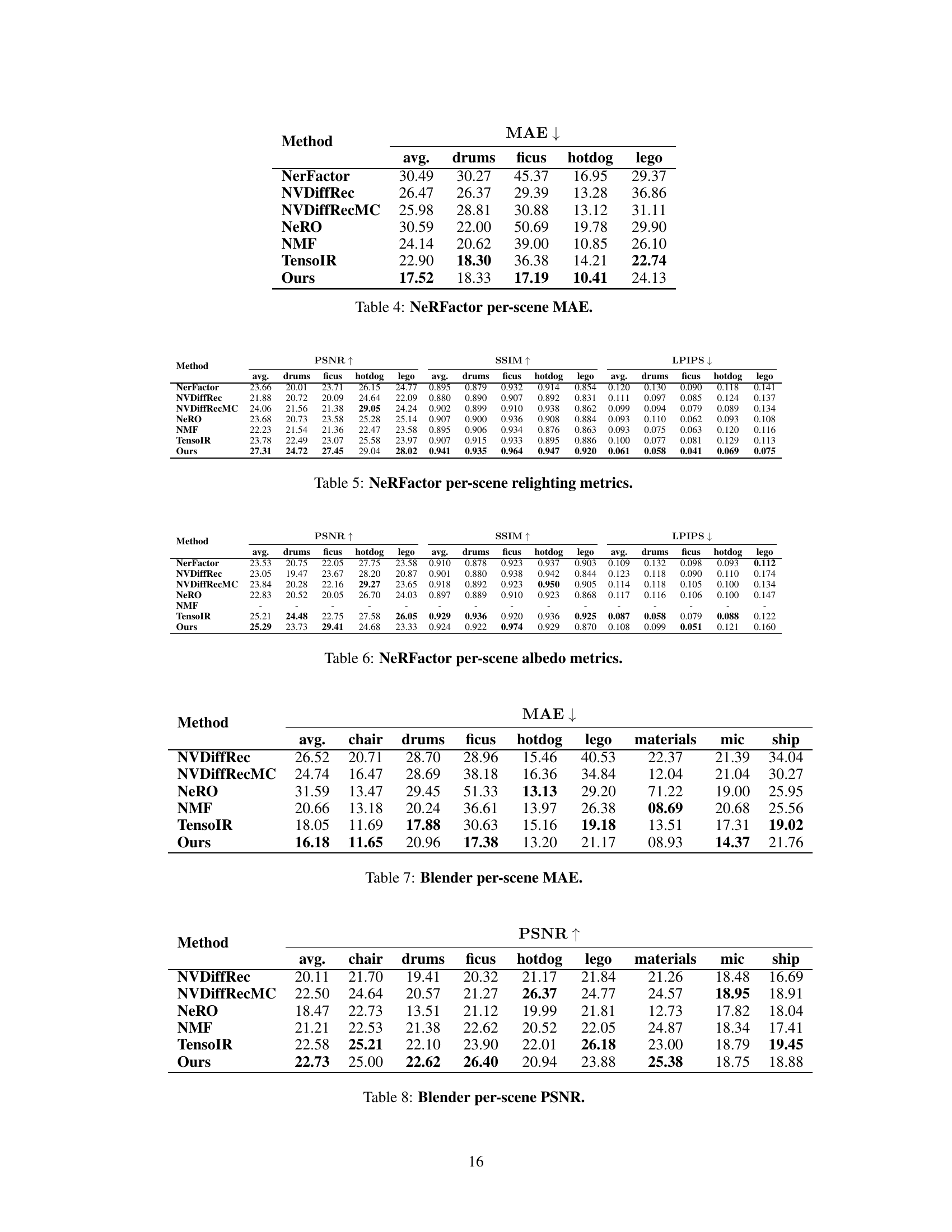
🔼 This table presents the Mean Absolute Error (MAE) for normals for each scene in the NeRFactor dataset. It compares the performance of the proposed method against several baselines across four scenes (‘drums’, ‘ficus’, ‘hotdog’, and ’lego’). Lower MAE values indicate better performance in estimating normals.
read the caption
Table 4: NeRFactor per-scene MAE.

🔼 This table presents a quantitative comparison of the proposed method against several state-of-the-art baselines on the NeRFactor dataset. Metrics include MAE, PSNR, SSIM, and LPIPS for normals, albedo, and relighting, as well as the runtime. The results demonstrate the competitive performance and efficiency of the proposed method.
read the caption
Table 1: NeRFactor metrics. We evaluate the reconstruction quality of our method against the baselines using 20 test images and 8 low-frequency illumination maps for each scene from the NeRFactor dataset. We scale albedo and relit images with a per-channel factor before computing metrics. Our method attains competitive performance across all metrics with a low runtime.

🔼 This table presents a quantitative comparison of the proposed method against several baselines on the NeRFactor dataset. Metrics include MAE, PSNR, SSIM, and LPIPS for normals, albedo, and relighting. The table shows that the proposed method achieves competitive performance across all metrics while having a faster runtime than most baselines.
read the caption
Table 1: NeRFactor metrics. We evaluate the reconstruction quality of our method against the baselines using 20 test images and 8 low-frequency illumination maps for each scene from the NeRFactor dataset. We scale albedo and relit images with a per-channel factor before computing metrics. Our method attains competitive performance across all metrics with a low runtime.

🔼 This table presents a comparison of the proposed method against several baselines on two datasets: Blender and Shiny Blender. The metrics used evaluate the quality of relighting reconstruction, including normal error. High-frequency illumination conditions were used to assess performance, and results demonstrate the superiority of the proposed method.
read the caption
Table 2: Blender and Shiny Blender metrics. We report the average of relighting reconstruction metrics and normal error for our extended Blender and Shiny Blender datasets. Metrics are computed as the average of 20 test views across 7 high-frequency illumination conditions for each scene. We scale images by a per-channel factor for relighting metrics. Our method outperforms the baselines across all metrics for the Blender dataset and has a higher PSNR for the Shiny Blender dataset.

🔼 This table presents a comparison of the proposed method against several baselines on two datasets: Blender and Shiny Blender. The metrics used evaluate the quality of relighting reconstruction and normal estimation. High-frequency illumination conditions were used, and image scaling was applied before metric calculations. The results show that the proposed method generally outperforms the baselines.
read the caption
Table 2: Blender and Shiny Blender metrics. We report the average of relighting reconstruction metrics and normal error for our extended Blender and Shiny Blender datasets. Metrics are computed as the average of 20 test views across 7 high-frequency illumination conditions for each scene. We scale images by a per-channel factor for relighting metrics. Our method outperforms the baselines across all metrics for the Blender dataset and has a higher PSNR for the Shiny Blender dataset.

🔼 This table presents a quantitative comparison of the proposed method against several baselines on the NeRFactor dataset. The metrics used evaluate the accuracy of normal prediction, albedo estimation, and relighting quality. The runtime of each method is also included. The table shows that the proposed method achieves competitive or better results across all metrics while being significantly faster.
read the caption
Table 1: NeRFactor metrics. We evaluate the reconstruction quality of our method against the baselines using 20 test images and 8 low-frequency illumination maps for each scene from the NeRFactor dataset. We scale albedo and relit images with a per-channel factor before computing metrics. Our method attains competitive performance across all metrics with a low runtime.

🔼 This table presents a quantitative comparison of the proposed method against several baseline methods on the NeRFactor dataset. The metrics used evaluate the quality of normal, albedo, and relighting predictions. The table shows that the proposed method achieves competitive or better performance across all metrics while maintaining a significantly lower runtime than most baselines.
read the caption
Table 1: NeRFactor metrics. We evaluate the reconstruction quality of our method against the baselines using 20 test images and 8 low-frequency illumination maps for each scene from the NeRFactor dataset. We scale albedo and relit images with a per-channel factor before computing metrics. Our method attains competitive performance across all metrics with a low runtime.

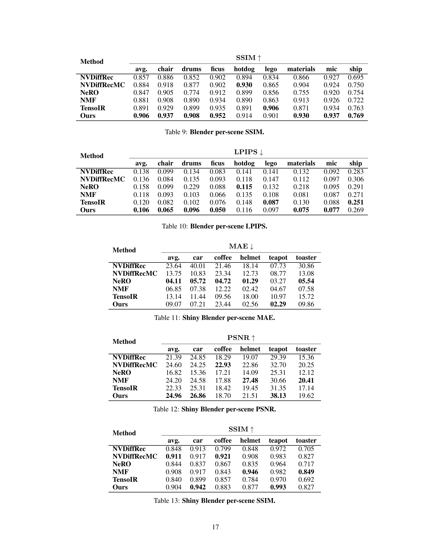
🔼 This table presents the Mean Absolute Error (MAE) for normal estimation on the Shiny Blender dataset. The MAE is a measure of the average difference between predicted and ground truth normal vectors at each pixel. Lower MAE values indicate better performance. The table breaks down the MAE across six different scenes within the Shiny Blender dataset: ‘car’, ‘coffee’, ‘helmet’, ’teapot’, and ’toaster’. The ‘avg.’ column represents the average MAE across all six scenes.
read the caption
Table 11: Shiny Blender per-scene MAE.

🔼 This table presents a comparison of the proposed method against several baselines on two datasets: Blender and Shiny Blender. The evaluation metrics include Mean Absolute Error (MAE) for normals, Peak Signal-to-Noise Ratio (PSNR) and Structural Similarity Index Measure (SSIM) for relighting, and Learned Perceptual Image Patch Similarity (LPIPS) for both relighting and normals. The results show that the proposed method achieves superior performance, particularly on the Blender dataset.
read the caption
Table 2: Blender and Shiny Blender metrics. We report the average of relighting reconstruction metrics and normal error for our extended Blender and Shiny Blender datasets. Metrics are computed as the average of 20 test views across 7 high-frequency illumination conditions for each scene. We scale images by a per-channel factor for relighting metrics. Our method outperforms the baselines across all metrics for the Blender dataset and has a higher PSNR for the Shiny Blender dataset.

🔼 This table presents the Structural Similarity Index Measure (SSIM) for relighting reconstruction on the Shiny Blender dataset. The SSIM values are calculated for each scene (car, coffee, helmet, teapot, toaster) and averaged across all scenes. Higher SSIM values indicate better reconstruction quality, with a score of 1 representing perfect similarity to the ground truth.
read the caption
Table 12: Shiny Blender per-scene SSIM.

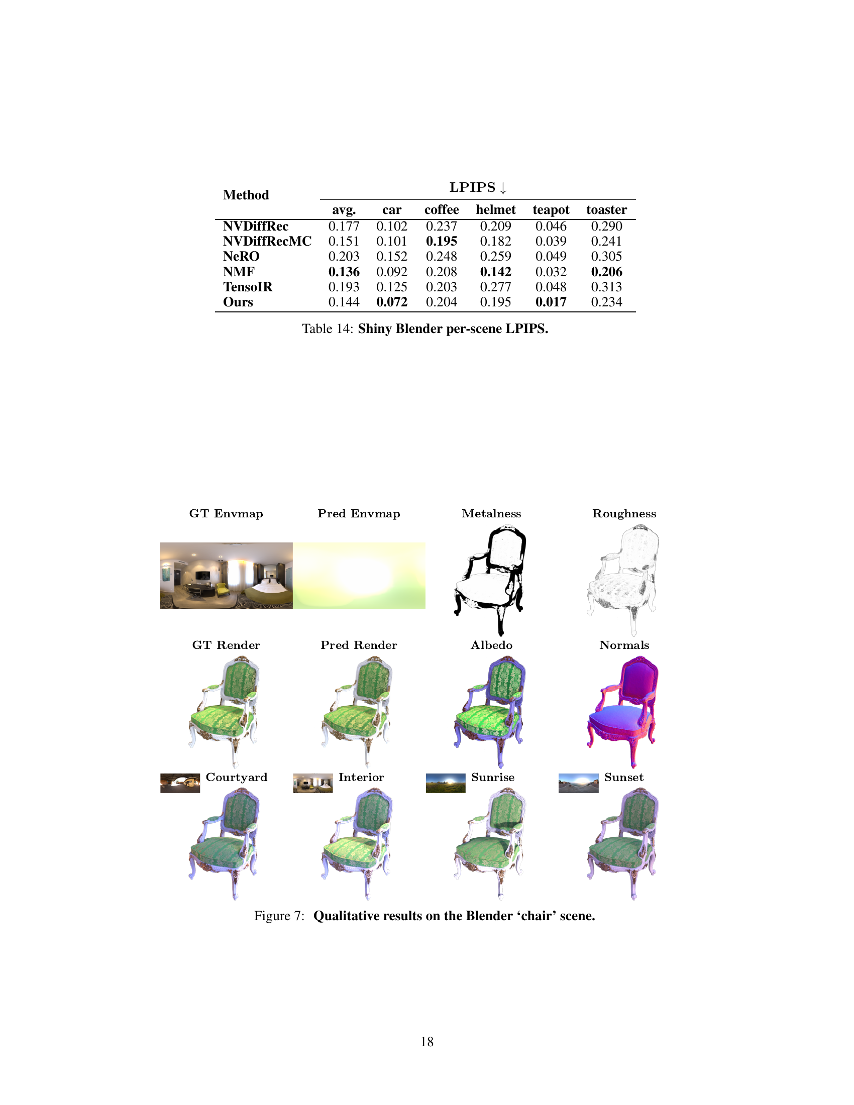
🔼 This table presents the Learned Perceptual Image Patch Similarity (LPIPS) scores for each scene in the Shiny Blender dataset. LPIPS is a perceptual metric that measures the dissimilarity between two images. Lower LPIPS scores indicate higher similarity. The table shows the average LPIPS across all test images for each scene (‘car’, ‘coffee’, ‘helmet’, ’teapot’, ’toaster’), as well as the overall average across all scenes and test images. The results are compared against several baseline methods (NVDiffRec, NVDiffRecMC, NeRO, NMF, TensoIR), showcasing the performance of the proposed ‘Ours’ method.
read the caption
Table 14: Shiny Blender per-scene LPIPS.
Full paper#
