TL;DR#
Understanding how neural networks function is hindered by the “black box” nature of their internal processes. Existing methods for interpreting neural activations have limitations in scope and often require researchers to predefine what information to extract. This is where InversionView shines. It addresses these challenges by focusing on the pre-image of activations, i.e., the inputs that yield similar activation patterns. By sampling from the pre-image, this method allows researchers to directly infer the information encoded by each activation vector.
InversionView is applied to several case studies, including character counting, indirect object identification, and 3-digit addition, using various models from small transformers to GPT-2. Results show that InversionView effectively reveals valuable information in activations, confirming the decoded information via causal intervention. It successfully uncovers both basic and complex information like token identity, position, counts, and abstract knowledge. This generalized approach significantly improves the interpretability of neural networks, providing a more comprehensive understanding of their decision-making processes and advancing AI safety research.
Key Takeaways#
Why does it matter?#
This paper is crucial for AI researchers because it introduces a novel method for interpreting neural networks, a persistent challenge in the field. InversionView offers a practical and general-purpose approach to understanding the information encoded in neural activations, moving beyond the limitations of existing methods. This opens exciting new avenues for researching AI safety, controllability, and the development of more explainable AI systems.
Visual Insights#
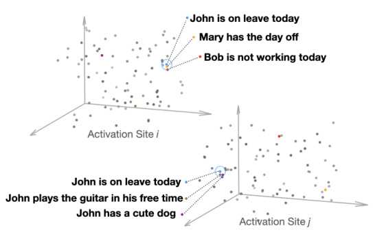
🔼 This figure from the Methodology section illustrates the concept of InversionView by showing how different activation sites in a neural network encode different types of information. The top panel shows an activation site that encodes the semantics of ‘being on leave’, while the bottom panel shows an activation site that encodes information about the subject of the sentence (John). The different colored points represent different input sentences, and their clustering demonstrates how similar inputs result in similar activations. This visualization helps explain how InversionView uses the geometry of the activation space to identify the information encoded in a given activation vector.
read the caption
Figure 1: Illustration of the geometry at two different activation sites, encoding different information about the input. Top: the semantics of being on leave are encoded. Bottom: the information that the subject of the input sentence is John is encoded.
🔼 This table summarizes the findings of the Indirect Object Identification (IOI) task using InversionView. It compares the information obtained using InversionView to the information and function described by Wang et al. [54]. Each row represents a different category of attention heads found in the IOI circuit, along with their function according to Wang et al. [54], the information captured by InversionView, and whether the results were consistent.
read the caption
Table 2: Column “Position” means the query activation is taken from that position. “S1+1” means the token right after S1. Rows are ordered according to the narration in the original paper. When we say “S name”, it means the the name of S in the query input, but the name is not necessarily S in the samples. This also applies to “IO name”. The information learned by InversionView which is different from the information suggested by Wang et al. [54] is in bold.
In-depth insights#
InversionView Intro#
The hypothetical ‘InversionView Intro’ section would likely introduce the core concept of InversionView, positioning it as a novel method to understand neural network inner workings. It would emphasize the black box nature of neural networks and the challenges in interpreting their internal representations. The introduction would highlight the significance of deciphering information encoded within neural activations and propose InversionView as a general-purpose solution. It would briefly touch upon existing methods for interpreting neural activations and their limitations, setting the stage for InversionView’s unique approach. The core novelty of InversionView might involve its focus on the pre-image of activations – the set of inputs producing similar activations – arguing that this pre-image directly embodies the information content. The introduction would likely hint at the practical application of InversionView, perhaps mentioning the use of a trained decoder model to sample from the pre-image and how this facilitates a deeper understanding of transformer model algorithms. Finally, a concise overview of the paper’s structure and the case studies used to demonstrate the efficacy of InversionView would conclude the introduction, promising valuable insights into the inner workings of neural networks.
Decoding Activations#
Decoding neural network activations is crucial for understanding their internal workings. This involves translating the high-dimensional vector representations into human-interpretable insights. InversionView, as presented in the research paper, offers a novel approach by focusing on the pre-image of activations—the set of inputs that produce similar activation patterns. This differs from techniques like supervised probes which rely on pre-defined tasks. Instead, InversionView leverages a trained decoder to sample inputs based on a given activation, revealing the underlying information encoded in these vectors. The method’s strength lies in its generality and applicability across diverse model architectures and tasks. It facilitates the discovery of algorithms implemented by the models by allowing researchers to examine the commonalities within this sampled pre-image. However, challenges include the scalability of sampling from potentially large input spaces and the inherent complexity of interpreting the decoded information. Nonetheless, InversionView demonstrates promise as a principled tool for gaining a deeper understanding of neural network behavior and deciphering the information content of their internal activations, ultimately paving the way for better model transparency and control.
Transformer Circuits#
The concept of “Transformer Circuits” represents a significant advancement in neural network interpretability. It posits that complex neural networks, particularly transformer models, can be understood not as monolithic black boxes, but rather as a collection of interconnected, modular circuits. These circuits, potentially consisting of attention heads, MLP layers, and other components, perform specific sub-computations. Understanding these circuits requires identifying the information flow and processing within each component and how they interact. This approach moves beyond simple visualization of activations to a deeper understanding of the underlying algorithmic processes. The success of this approach hinges on the ability to identify the functional roles of individual circuits by observing how they transform input information. By dissecting the network into smaller, more manageable units, the Transformer Circuits framework makes the internal workings of large, deep networks more comprehensible. Furthermore, this approach facilitates targeted interventions and analyses which can provide detailed explanations for the model’s decisions and behavior. Challenges include the complexity of identifying and mapping these circuits, and the variability in behavior that may emerge from interactions between circuits.
InversionView Limits#
InversionView, while powerful, has limitations. Scalability is a concern; exhaustively searching the preimage becomes computationally expensive with high-dimensional data and large models. The reliance on a trained decoder introduces an additional layer of complexity and potential bias, and the decoder’s accuracy directly impacts the reliability of the results. Moreover, the method’s reliance on a threshold parameter requires careful consideration as it impacts the granularity and scope of the information revealed. The success of InversionView also depends on the representational geometry of the activations, which is model-specific and may not always be intuitive or consistent. Finally, interpreting the preimages themselves, while potentially aided by LLMs, remains a labor-intensive and subjective process, highlighting the need for further automation to fully harness its potential.
Future Directions#
Future research could explore several promising avenues. Scaling InversionView to larger models and datasets is crucial, requiring efficient methods for handling high-dimensional activation spaces and potentially more sophisticated decoder architectures. Automating the interpretation process further, perhaps by leveraging large language models to analyze the generated samples and formulate hypotheses, would significantly increase efficiency and scalability. Investigating the applicability of InversionView across different neural network architectures and modalities, such as vision and audio, would broaden its impact and reveal potential insights into how information is processed in various contexts. A deeper exploration of the relationship between InversionView and other interpretability methods, such as causal intervention and activation patching, may lead to more powerful and comprehensive techniques. Lastly, investigating how different distance metrics and threshold selection techniques influence the results and exploring optimal choices for different scenarios and model types would be valuable.
More visual insights#
More on figures
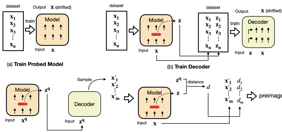
🔼 This figure illustrates the three main steps of InversionView. (a) shows the training of a probed model which is used to obtain activations. (b) shows how these activations along with their corresponding inputs are cached and used to train the decoder. (c) shows the process of interpreting a specific activation by sampling inputs from the trained decoder and evaluating distances in the original model to determine preimage.
read the caption
Figure 2: (a) The probed model is trained on language modeling objective. (b) Given a trained probed model, we first cache the internal activations z together with their corresponding inputs and activation site indices (omitted in the figure for brevity), then use them to train the decoder. The decoder is trained with language modeling objective, while being able to attend to z. (c) When interpreting a specific query activation zq, we give it to the decoder, which generates possible inputs auto-regressively. We then evaluate the distances on the original probed model.
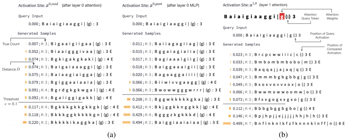
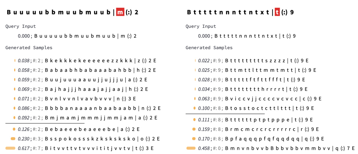
🔼 This figure demonstrates InversionView’s application to a character counting task. It showcases how the model processes and forgets information across different layers (MLP and attention). The visualizations highlight how the model’s activations encode information about the count of specific characters and how this count information is preserved even as other features are dropped.
read the caption
Figure 3: InversionView on Character Counting Task. The model counts how often the target character (after 'l') occurs in the prefix (before 'l'). B and E denote beginning and end of sequence tokens. The query activation conditions the decoder to generate samples capturing its information content. We show non-cherrypicked samples inside and outside the e-preimage (€ = 0.1) at three activation sites on the same query input. Distance for each sample is calculated between activations corresponding to the parenthesized characters in the query input and the sample. 'True count' indicates the correct count of the target character in the samples (decoder may generate incorrect counts). (a) MLP layer amplifies count information. Comparing the distances before (left) and after (right) the MLP, we see that samples with diverging counts become much more distant from the query activation. (b) In the next layer (':' exclusively attends to target character – copying information from residual stream of target character to the residual stream of ':'), the count is retained but the identity of the target character is no longer encoded ('c', 'm', etc. instead of 'g'), as it is no longer relevant for the predicting the count. Therefore, observing the generations informs us of the activations' content and how it changes across activation sites.

🔼 This figure shows the results of activation patching experiments for character counting and IOI tasks. The top panels (a) illustrate how patching specific activations in the character counting model affects the model’s prediction accuracy. This validates the hypothesis of information flow derived from InversionView. The bottom panels (b) demonstrate the application of InversionView to an attention head in the IOI task. By sampling from the decoder conditioned on the activation, the common information among the generated samples reveals that the head encodes a specific name.
read the caption
Figure 4: (a) Character Counting. Activation patching results show that ate and a1,0 play crucial roles in prediction, as hypothesized based on Figure 3 and Sec. 3.3. In contrast examples, only one character differs. Top: We patch activations cumulatively from left to right. We can see patching ate accounts for the whole effect, and when a¿º is already patched, patching a1,0 has almost no effect. Bottom: On the other hand, if we patch cumulatively from right to left, a1,0 accounts for the whole effect while patching a has no effect if a¹,0 has been patched. So we verified that a1,0 solely relies on ate a and this path is the one by which the model performs precise counting. The patching effect is averaged across the whole test set. (b) IOI. Inversion View applied to Name Mover Head 9.9 at 'to'; we fix the compared position to “to”. Throughout the e-preimage, “Justin” appears as the IO, revealing that the head encodes this name. This interpretation is confirmed across query inputs.

🔼 The figure shows the information flow diagrams for predicting digits in a 3-digit addition task, inferred using InversionView. It visually depicts how information is processed in the model’s different layers and heads. The diagrams are simplified to represent only the most stable and frequently observed paths during training. They show which parts of the input influence the prediction of each digit of the output.
read the caption
Figure 31: The information flow diagrams for predicting the digits in answer. F1 and S1 are aligned, F2 and S2 are aligned, and so forth. Color of the lines represents the information being routed, and alternating color represents a mixture of information. The computation is done from left to right (or simultaneously during training), and from bottom to top in each sub-figure. Note that the figure represents what information we find in activation, rather than the information being used by the model. Also note that the graphs are based on our qualitative examination using InversionView and attention pattern, and are an approximate representation of reality. We keep those stable paths that almost always occur. Inconsistently present paths such as routing the ones place when predicting A1 are not shown.
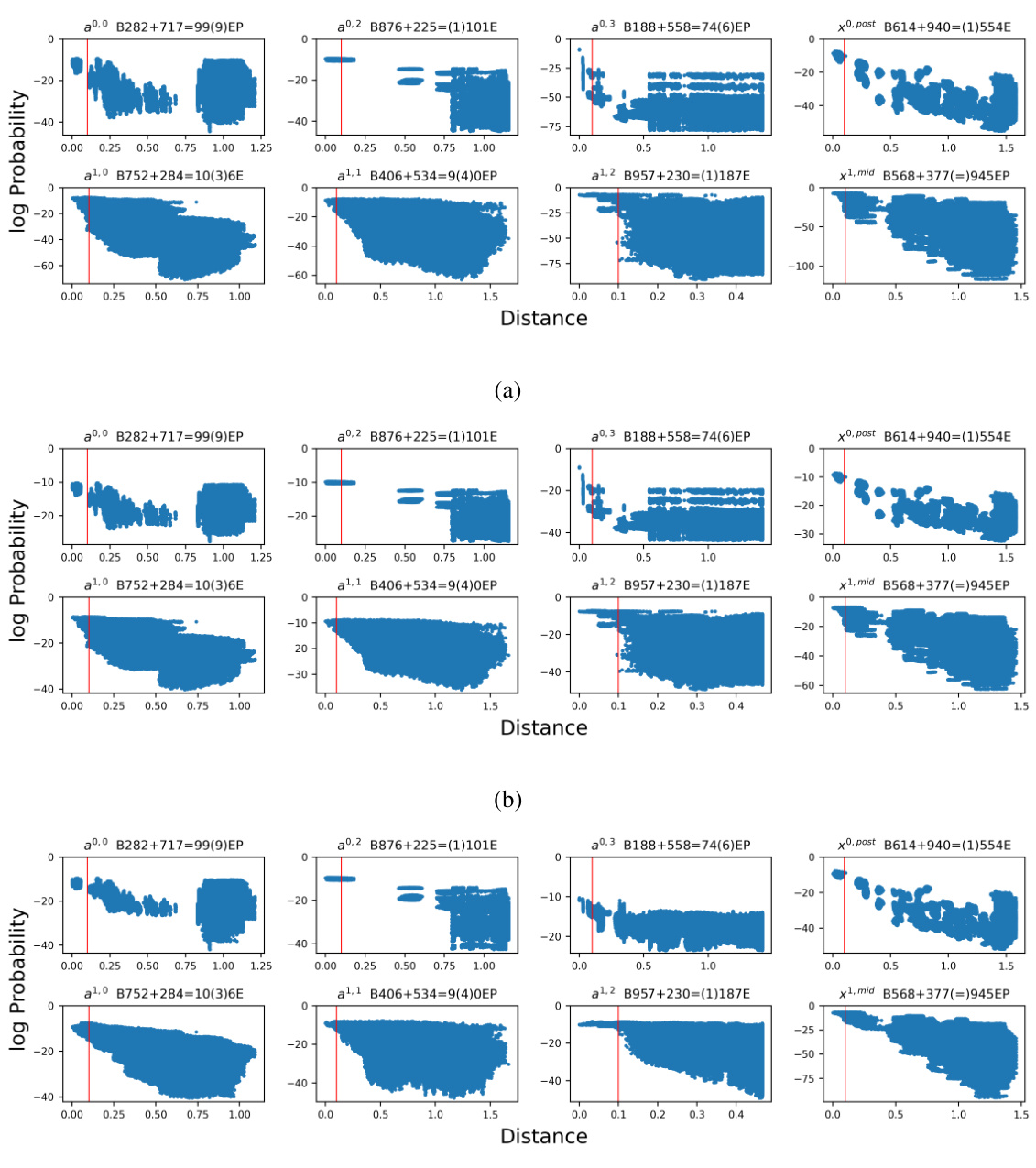
🔼 This figure shows the exhaustive verification of the decoder’s completeness for 8 random query activations in the 3-digit addition task. It uses scatter plots to visualize the relationship between log-probability of inputs (y-axis) and the distance to the query activation (x-axis), demonstrating that inputs within the e-preimage have higher probabilities than those outside. The impact of temperature and noise on probability is also shown.
read the caption
Figure 11: Addition Task: Exhaustive verification of the decoder's completeness for 8 random query activation. Failure of completeness would mean that some inputs result in an activation very close to the query activation but nonetheless are assigned very small probability. Here, we show that this does not happen, by verifying that all inputs within the e-preimage are assigned higher probability by the decoder than most other inputs. We also show that by increasing the temperature and adding random noise, we can increase the probability of inputs near the boundary of e-preimage. Each sub-figure – (a), (b), (c) – contains 8 scatter plots, each of which contains 810000 dots representing all input sequences in the 3-digit addition task. The y-axis of scatter plots is the log-probability of the input sequence given by the decoder (which reads the query activation), the x-axis is the distance between the query input and the input sequence. As before, distance is measured by the normalized Euclidean distance between the query activation (the activation site, query input, and selected position are shown in the scatter plot title) and the most similar activation along the sequence axis. In addition, the red vertical line represents the threshold e, which is 0.1 in the case study. (a) Temperature т = 1.0, no noise is added. (b) Temperature r = 2.0, no noise is added. (c) Temperature т = 1.0, noise coefficient η = 0.1 (See Appendix A.2 for explanation of n).
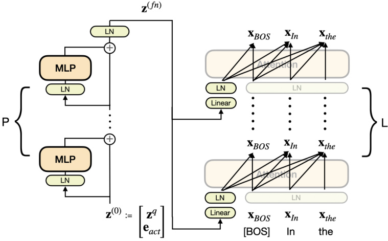
🔼 This figure illustrates the architecture of the decoder model used in the InversionView method. The model is a decoder-only transformer with added MLP layers to process the query activation. The query activation (zq) is first concatenated with an activation site embedding (eact) and then passed through multiple MLP layers with residual connections. The output (z(fn)) is then used to condition the attention layers in each layer of the transformer. The transparency of certain blocks highlights that some parts of the architecture were inherited from the original decoder-only transformer.
read the caption
Figure 12: The decoder model architecture used in this paper. The query activation is processed by a stack of MLP layers before being available as part of the context in attention layers. We use transparent blocks to represent model components inherited from original decoder-only transformer model.
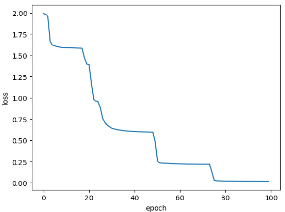
🔼 The figure shows the training loss curve for the character counting task. The x-axis represents the training epoch, and the y-axis represents the average training loss. The loss curve shows a sharp decrease initially, followed by a series of smaller decreases and plateaus. The stair-step pattern in the curve might be indicative of the learning algorithm’s behavior in navigating the loss landscape.
read the caption
Figure 13: Training loss of the Character Counting task. Each data point is the averaged loss over an epoch.

🔼 This figure shows the results of a causal intervention experiment where the effect of different activations in the character counting model was investigated using activation patching. The experiment involved patching a series of activations, starting from either the beginning or end of the model’s layers. The results are presented as line plots showing the change in logit difference (LD) between the original and contrast inputs as each additional activation is patched. The goal is to determine the causal influence of each activation on the model’s prediction, providing evidence for the proposed algorithm.
read the caption
Figure 16: Results of activation patching for model trained on character counting task. Same figure as 4a with intermediate steps of calculation shown using line plot. Note that the gray lines correspond to the y-axis on the right. In contrast examples, only one character differs. LD stands for logit difference between the original count and the count in the contrast example. LDpch and LDorig correspond to the LD with and without patching, respectively. Top: We patch activations cumulatively from left to right, flipping the sign of LD. The “none” on the left end of x-axis denotes the starting point, i.e., nothing is patched. Bottom: We patch from right to left. Similarly, “none” on the right end of x-axis denotes the starting point.

🔼 This figure shows the results of an ablation study using activation patching. The experiment systematically patches different activations within the model, from left-to-right and right-to-left, while tracking the effect on the logit difference (LD) between the original count and a contrast example (differing by one character). The results help to verify the causal influence of specific activations in the character-counting process by demonstrating which patches substantially change the LD. The figure shows how intermediate activations contribute to the final model’s prediction, clarifying the flow of information in the model.
read the caption
Figure 16: Results of activation patching for model trained on character counting task. Same figure as 4a with intermediate steps of calculation shown using line plot. Note that the gray lines correspond to the y-axis on the right. In contrast examples, only one character differs. LD stands for logit difference between the original count and the count in the contrast example. LDpch and LDorig correspond to the LD with and without patching, respectively. Top: We patch activations cumulatively from left to right, flipping the sign of LD. The “none” on the left end of x-axis denotes the starting point, i.e., nothing is patched. Bottom: We patch from right to left. Similarly, “none” on the right end of x-axis denotes the starting point.
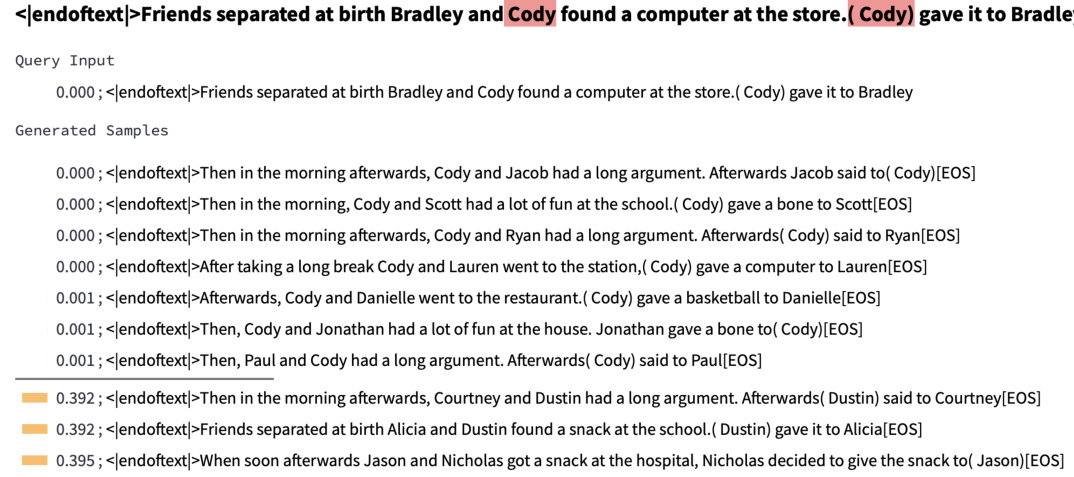
🔼 This figure shows the results of applying InversionView to the Duplicate Token Head 0.1 in the IOI task. The caption indicates that the information about the subject (S) is present in the head’s output. The figure’s contents show example generated inputs from a decoder model trained on the activation of the head, which are consistent with the hypothesis that this head encodes the subject’s name. The generated inputs vary but they all contain the same name ‘Justin’ as the indirect object (IO).
read the caption
Figure 20: e-preimage of Duplicate Token Head 0.1. S name is contained in head output.

🔼 This figure shows the results of applying InversionView to an IOI task using a specific attention head. The caption highlights that the head’s activation encodes the position of the last occurrence of the token in parentheses (the indirect object in the IOI sentence) but not the token’s identity itself. In other words, the head seems to ‘remember’ where the indirect object was mentioned previously in the sentence, not what the indirect object was.
read the caption
Figure 21: e-preimage of Induction Head 5.5. Position – but not identity – of the current token (token in parenthesis)'s last occurrence is contained in head output.

🔼 This figure shows the Indirect Object Identification (IOI) circuit in GPT-2 small, which was discovered by Wang et al. [54]. It illustrates the flow of information through different types of attention heads in the model during the IOI task. The different head types (Previous Token Heads, Duplicate Token Heads, Induction Heads, S-Inhibition Heads, Negative Name Mover Heads, Name Mover Heads, Backup Name Mover Heads) are categorized by color and grouped in boxes. The figure illustrates the sequence of information processing in the model by indicating how the information flows between heads to ultimately identify the indirect object.
read the caption
Figure 22: IOI circuit in GPT-2 small. Figure 2 from [54]

🔼 The figure shows a plot of the training loss versus the number of epochs for the character counting task. The loss decreases rapidly in the first few epochs and then plateaus, indicating that the model is learning effectively. The stair-like pattern in the loss curve might indicate that the model is learning in stages.
read the caption
Figure 13: Training loss of the Character Counting task. Each data point is the averaged loss over an epoch.

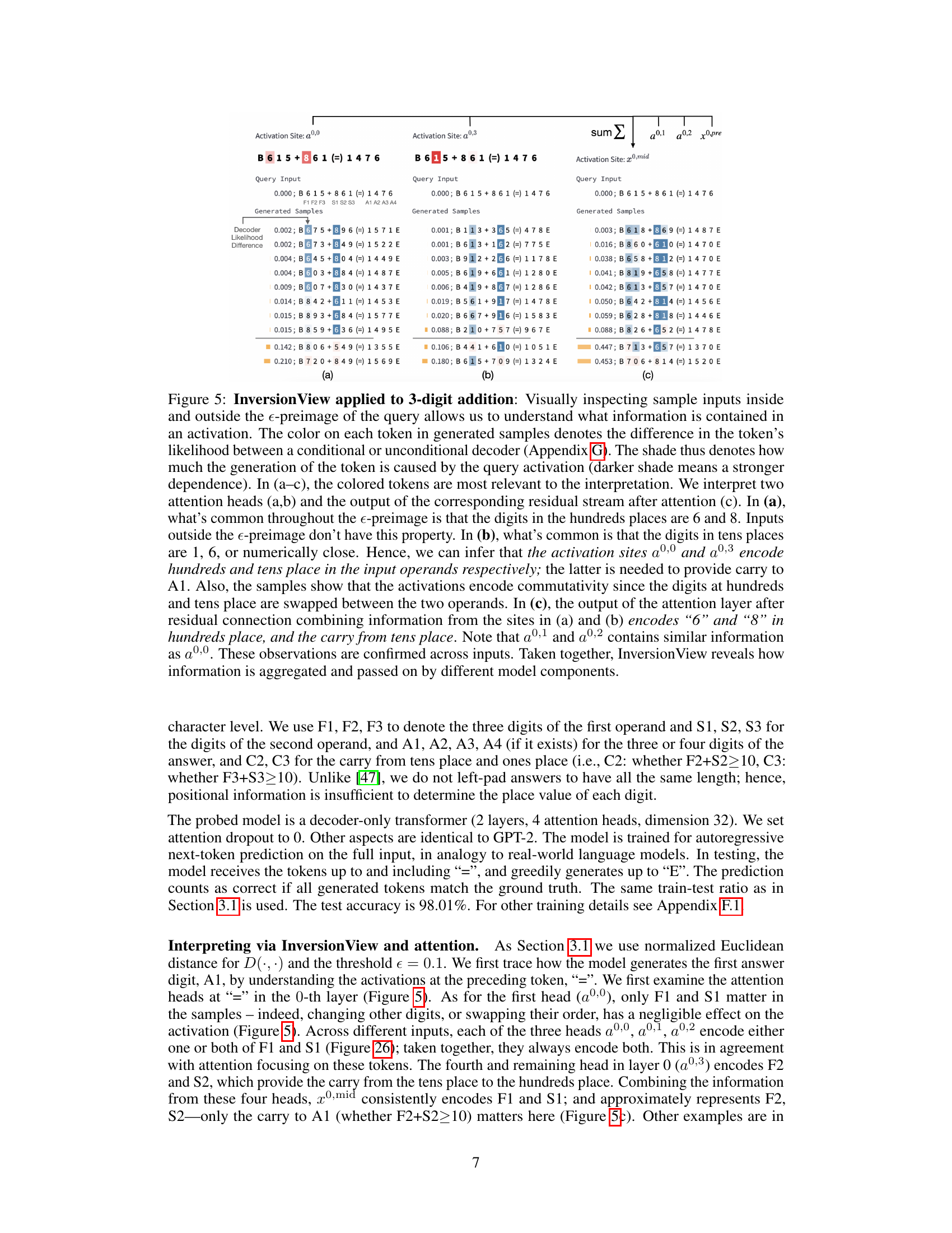
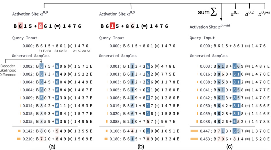
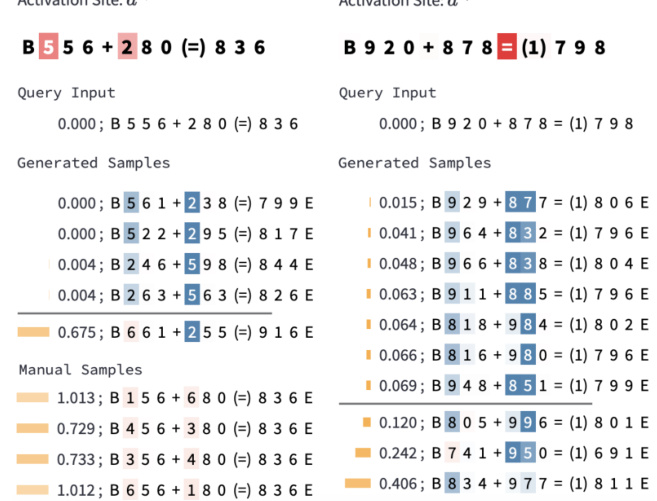
🔼 This figure shows how InversionView is used to interpret the information encoded in different activation sites of a 3-digit addition model. By analyzing the samples within and outside the e-preimage of specific activation sites, the authors identify which aspects of the input (hundreds, tens, ones digits; carry) are encoded by each site. The color-coding of tokens in generated samples highlights the influence of the query activation on token likelihood. The figure demonstrates how information flows through different layers of the model.
read the caption
Figure 5: InversionView applied to 3-digit addition: Visually inspecting sample inputs inside and outside the e-preimage of the query allows us to understand what information is contained in an activation. The color on each token in generated samples denotes the difference in the token's likelihood between a conditional or unconditional decoder (Appendix G). The shade thus denotes how much the generation of the token is caused by the query activation (darker shade means a stronger dependence). In (a–c), the colored tokens are most relevant to the interpretation. We interpret two attention heads (a, b) and the output of the corresponding residual stream after attention (c). In (a), what's common throughout the e-preimage is that the digits in the hundreds places are 6 and 8. Inputs outside the e-preimage don't have this property. In (b), what's common is that the digits in tens places are 1, 6, or numerically close. Hence, we can infer that the activation sites a0,0 and a0,3 encode hundreds and tens place in the input operands respectively; the latter is needed to provide carry to A1. Also, the samples show that the activations encode commutativity since the digits at hundreds and tens place are swapped between the two operands. In (c), the output of the attention layer after residual connection combining information from the sites in (a) and (b) encodes “6” and “8” in hundreds place, and the carry from tens place. Note that a0,1 and a0,2 contains similar information as a0,0. These observations are confirmed across inputs. Taken together, InversionView reveals how information is aggregated and passed on by different model components.

🔼 This figure demonstrates InversionView’s application to a character counting task. It shows how the model processes and retains information about the count of a specific character, even as other aspects of the input change. The figure highlights the role of the MLP layer in amplifying count information and how this information is subsequently abstracted and propagated through different layers of the transformer model.
read the caption
Figure 3: InversionView on Character Counting Task. The model counts how often the target character (after 'l') occurs in the prefix (before 'l'). B and E denote beginning and end of sequence tokens. The query activation conditions the decoder to generate samples capturing its information content. We show non-cherrypicked samples inside and outside the e-preimage (€ = 0.1) at three activation sites on the same query input. Distance for each sample is calculated between activations corresponding to the parenthesized characters in the query input and the sample. 'True count' indicates the correct count of the target character in the samples (decoder may generate incorrect counts). (a) MLP layer amplifies count information. Comparing the distances before (left) and after (right) the MLP, we see that samples with diverging counts become much more distant from the query activation. (b) In the next layer (':' exclusively attends to target character – copying information from residual stream of target character to the residual stream of ':'), the count is retained but the identity of the target character is no longer encoded ('c', 'm', etc. instead of 'g'), as it is no longer relevant for the predicting the count. Therefore, observing the generations informs us of the activations' content and how it changes across activation sites.

🔼 This figure demonstrates the InversionView method applied to a character counting task. It shows examples of generated samples from a decoder conditioned on activations from three different layers of a transformer network. The samples illustrate how the model processes and retains information about the count of a specific character, even as other aspects of the input change. The before and after MLP comparisons showcase how an MLP layer amplifies count information, making it more prominent in the activation’s representation. It also illustrates how the count information is transferred to a colon token in a subsequent layer, while losing information about the target character’s identity.
read the caption
Figure 3: InversionView on Character Counting Task. The model counts how often the target character (after 'l') occurs in the prefix (before 'l'). B and E denote beginning and end of sequence tokens. The query activation conditions the decoder to generate samples capturing its information content. We show non-cherrypicked samples inside and outside the e-preimage (€ = 0.1) at three activation sites on the same query input. Distance for each sample is calculated between activations corresponding to the parenthesized characters in the query input and the sample. 'True count' indicates the correct count of the target character in the samples (decoder may generate incorrect counts). (a) MLP layer amplifies count information. Comparing the distances before (left) and after (right) the MLP, we see that samples with diverging counts become much more distant from the query activation. (b) In the next layer (':' exclusively attends to target character – copying information from residual stream of target character to the residual stream of ':'), the count is retained but the identity of the target character is no longer encoded ('c', 'm', etc. instead of 'g'), as it is no longer relevant for the predicting the count. Therefore, observing the generations informs us of the activations' content and how it changes across activation sites.
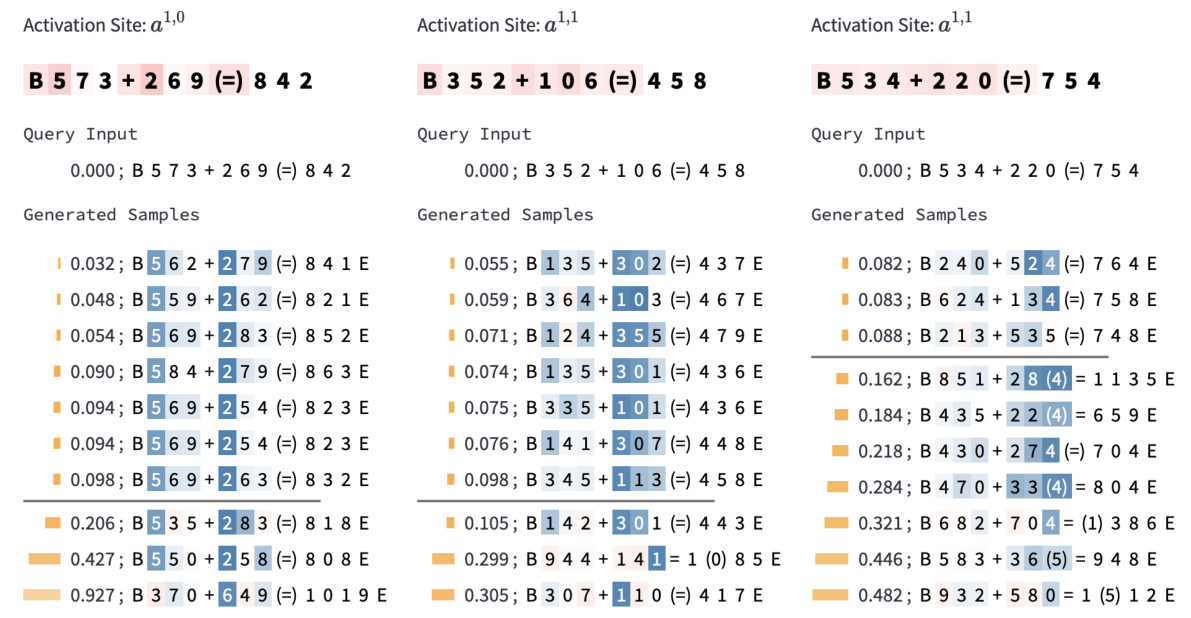
🔼 This figure shows how InversionView is used to understand what information is encoded in different activation sites of a 3-digit addition task. It uses color-coding to show the likelihood of tokens generated from a decoder model, revealing how information is aggregated and passed between different layers and components of the model.
read the caption
Figure 5: InversionView applied to 3-digit addition: Visually inspecting sample inputs inside and outside the e-preimage of the query allows us to understand what information is contained in an activation. The color on each token in generated samples denotes the difference in the token's likelihood between a conditional or unconditional decoder (Appendix G). The shade thus denotes how much the generation of the token is caused by the query activation (darker shade means a stronger dependence). In (a–c), the colored tokens are most relevant to the interpretation. We interpret two attention heads (a, b) and the output of the corresponding residual stream after attention (c). In (a), what's common throughout the e-preimage is that the digits in the hundreds places are 6 and 8. Inputs outside the e-preimage don't have this property. In (b), what's common is that the digits in tens places are 1, 6, or numerically close. Hence, we can infer that the activation sites a0,0 and a0,3 encode hundreds and tens place in the input operands respectively; the latter is needed to provide carry to A1. Also, the samples show that the activations encode commutativity since the digits at hundreds and tens place are swapped between the two operands. In (c), the output of the attention layer after residual connection combining information from the sites in (a) and (b) encodes “6” and “8” in hundreds place, and the carry from tens place. Note that a0,1 and a0,2 contains similar information as a0,0. These observations are confirmed across inputs. Taken together, InversionView reveals how information is aggregated and passed on by different model components.
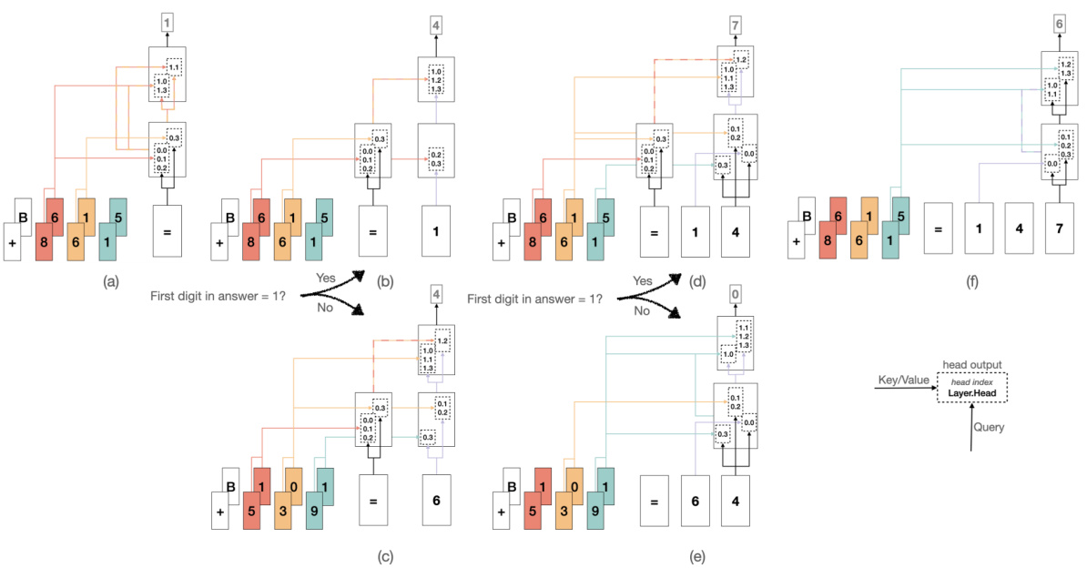
🔼 This figure shows the information flow diagrams for predicting digits in the answer of the 3-digit addition task. The diagrams illustrate how information is processed and routed through the network. The color-coding represents the type of information being passed, while alternating colors signify a combination of information types. The flow is depicted from left to right, simulating the model’s processing, and from bottom to top within each diagram. This is an approximation based on qualitative analysis using InversionView and attention patterns; consistently occurring paths are retained, but less frequent paths are omitted for clarity.
read the caption
Figure 31: The information flow diagrams for predicting the digits in answer. F1 and S1 are aligned, F2 and S2 are aligned, and so forth. Color of the lines represents the information being routed, and alternating color represents a mixture of information. The computation is done from left to right (or simultaneously during training), and from bottom to top in each sub-figure. Note that the figure represents what information we find in activation, rather than the information being used by the model. Also note that the graphs are based on our qualitative examination using InversionView and attention pattern, and are an approximate representation of reality. We keep those stable paths that almost always occur. Inconsistently present paths such as routing the ones place when predicting A1 are not shown.
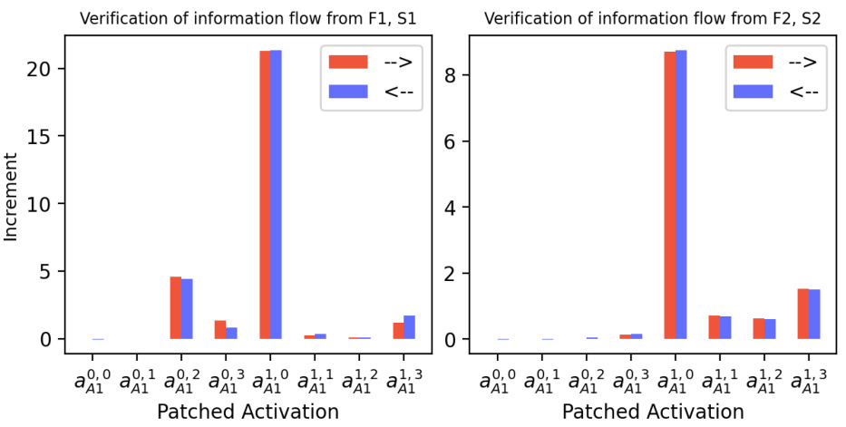
🔼 This figure shows the causal verification results for the information flow when predicting A2 given A1=1. Two causal intervention experiments were conducted: one changing F1 and S1, the other changing F2 and S2. The results support the information flow diagram in Figure 31b, demonstrating that the model uses the hundreds and tens digits to predict A2 when A1=1. The study ensured that contrast examples always satisfy F1+S1≥10.
read the caption
Figure 32: Causal verification results for the information flow in sub-figure (b) in Figure 31: predicting A2 when A1=1. We only consider data in Xorig where A1=1. The constructed contrast data Xcon also satisfies this constraint. Left: Tchg = {F1, S1}. Right: Tchg = {F2, S2}. Note that the included data from Xorig all satisfy F1+S1≥10, because, if F1+S1=9 and A1=1, no contrast example obtained by changing F2 and S2 would satisfy the constraint. The results confirm that information about the digits in hundreds and tens places is routed through the paths that we hypothesized based on InversionView in Figure 31b.
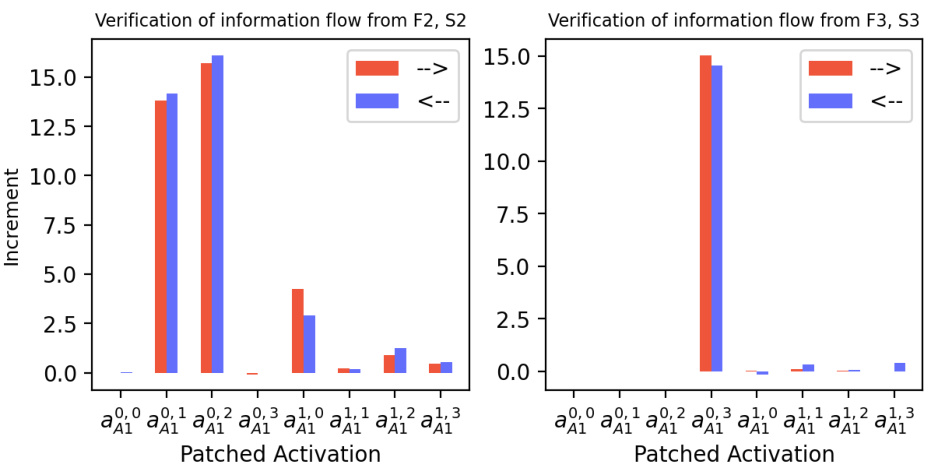
🔼 This figure shows the results of causal intervention experiments used to verify the information flow diagram shown in Figure 31(b). The experiments confirm that information about the digits in hundreds and tens places is correctly routed by the model via the paths hypothesized in Figure 31(b). The causal verification is done by comparing the logit difference between the original count and the count in a contrast example with and without patching of specific activations.
read the caption
Figure 32: Causal verification results for the information flow in sub-figure (b) in Figure 31: predicting A2 when A1=1. We only consider data in xorig where A1=1. The constructed contrast data xcon also satisfies this constraint. Left: Tchg = {F1, S1}. Right: Tchg = {F2, S2}. Note that the included data from xorig all satisfy F1+S1≥10, because, if F1+S1=9 and A1=1, no contrast example obtained by changing F2 and S2 would satisfy the constraint. The results confirm that information about the digits in hundreds and tens places is routed through the paths that we hypothesized based on InversionView in Figure 31b.

🔼 This figure demonstrates InversionView’s application to a character counting task. It shows how the model processes and retains information about the frequency of a target character. The figure analyzes activations at three different points within the model’s architecture (before and after an MLP layer, and in a subsequent attention layer) and illustrates how the model’s representation of the character count and identity evolves.
read the caption
Figure 3: InversionView on Character Counting Task. The model counts how often the target character (after 'l') occurs in the prefix (before 'l'). B and E denote beginning and end of sequence tokens. The query activation conditions the decoder to generate samples capturing its information content. We show non-cherrypicked samples inside and outside the e-preimage (€ = 0.1) at three activation sites on the same query input. Distance for each sample is calculated between activations corresponding to the parenthesized characters in the query input and the sample. 'True count' indicates the correct count of the target character in the samples (decoder may generate incorrect counts). (a) MLP layer amplifies count information. Comparing the distances before (left) and after (right) the MLP, we see that samples with diverging counts become much more distant from the query activation. (b) In the next layer (':' exclusively attends to target character – copying information from residual stream of target character to the residual stream of ':'), the count is retained but the identity of the target character is no longer encoded ('c', 'm', etc. instead of 'g'), as it is no longer relevant for the predicting the count. Therefore, observing the generations informs us of the activations' content and how it changes across activation sites.
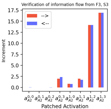
🔼 This figure shows the results of causal intervention experiments to verify the information flow for predicting A2 when A1=1. The experiments used activation patching to measure the causal effect of different activations on the model’s prediction. The results support the hypothesis, generated by InversionView, about which paths are responsible for routing information about the digits in hundreds and tens places.
read the caption
Figure 32: Causal verification results for the information flow in sub-figure (b) in Figure 31: predicting A2 when A1=1. We only consider data in Xorig where A1=1. The constructed contrast data Xcon also satisfies this constraint. Left: Tchg = {F1, S1}. Right: Tchg = {F2, S2}. Note that the included data from Xorig all satisfy F1+S1≥10, because, if F1+S1=9 and A1=1, no contrast example obtained by changing F2 and S2 would satisfy the constraint. The results confirm that information about the digits in hundreds and tens places is routed through the paths that we hypothesized based on InversionView in Figure 31b.
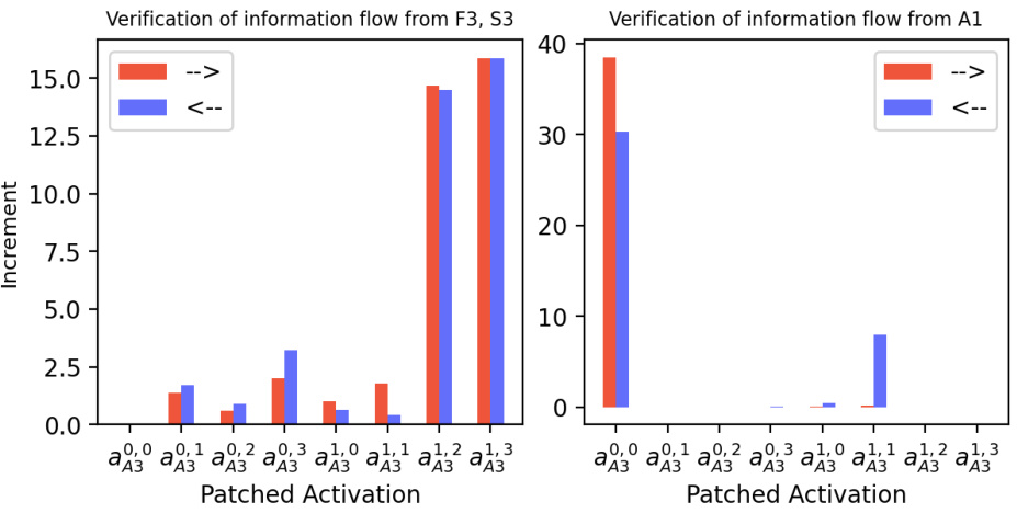
🔼 The figure shows causal verification results for the information flow when predicting A2 given that A1 is 1. It uses activation patching, comparing results when patching from left-to-right and right-to-left, with contrasts on F1/S1 and F2/S2 respectively. Results confirm information flow hypotheses based on InversionView.
read the caption
Figure 32: Causal verification results for the information flow in sub-figure (b) in Figure 31: predicting A2 when A1=1. We only consider data in Xorig where A1=1. The constructed contrast data Xcon also satisfies this constraint. Left: Tchg = {F1, S1}. Right: Tchg = {F2, S2}. Note that the included data from Xorig all satisfy F1+S1≥10, because, if F1+S1=9 and A1=1, no contrast example obtained by changing F2 and S2 would satisfy the constraint. The results confirm that information about the digits in hundreds and tens places is routed through the paths that we hypothesized based on InversionView in Figure 31b.
🔼 This figure demonstrates the application of InversionView to the Name Mover Head 9.9 at the word ’to’. Unlike a previous figure (Figure 4b), the position that minimizes the distance metric D(·, ·) is explicitly indicated in parentheses. The figure highlights that this head not only copies the name ‘Justin’ in the specific context of the indirect object identification (IOI) task but also copies it in other similar contexts, showing its broader function within the language model.
read the caption
Figure 38: InversionView applied to Name Mover Head 9.9 at 'to'. Unlike Figure 4b, here the position minimizing D(·, ·) is in parentheses. The head also copies the name “Justin” in other circumstances, e.g., at “gave”. The name “Justin” is always contained
🔼 This figure shows the results of applying InversionView to a character counting task. It demonstrates how the model processes and retains information about the count of a specific character, even as other aspects of the input change. The figure highlights the role of the MLP layer in amplifying count information and how information is abstracted as it flows through different layers. Subfigure (a) shows how the MLP layer increases the distance between samples with different counts from the query activation, enhancing count information. Subfigure (b) showcases how the next layer focuses specifically on the count, losing the target character’s identity.
read the caption
Figure 3: InversionView on Character Counting Task. The model counts how often the target character (after 'l') occurs in the prefix (before 'l'). B and E denote beginning and end of sequence tokens. The query activation conditions the decoder to generate samples capturing its information content. We show non-cherrypicked samples inside and outside the e-preimage (€ = 0.1) at three activation sites on the same query input. Distance for each sample is calculated between activations corresponding to the parenthesized characters in the query input and the sample. 'True count' indicates the correct count of the target character in the samples (decoder may generate incorrect counts). (a) MLP layer amplifies count information. Comparing the distances before (left) and after (right) the MLP, we see that samples with diverging counts become much more distant from the query activation. (b) In the next layer (':' exclusively attends to target character – copying information from residual stream of target character to the residual stream of ':'), the count is retained but the identity of the target character is no longer encoded ('c', 'm', etc. instead of 'g'), as it is no longer relevant for the predicting the count. Therefore, observing the generations informs us of the activations' content and how it changes across activation sites.
🔼 This figure demonstrates InversionView’s application to a character counting task using a small transformer model. It shows how the model processes and retains information about the count of a specific character, even while losing other details about the character’s identity. The figure compares the distances between activations before and after an MLP layer, and it highlights the transition of information to a subsequent layer which focuses only on the character count, abstracting away the character’s identity.
read the caption
Figure 3: InversionView on Character Counting Task. The model counts how often the target character (after 'l') occurs in the prefix (before 'l'). B and E denote beginning and end of sequence tokens. The query activation conditions the decoder to generate samples capturing its information content. We show non-cherrypicked samples inside and outside the e-preimage (€ = 0.1) at three activation sites on the same query input. Distance for each sample is calculated between activations corresponding to the parenthesized characters in the query input and the sample. 'True count' indicates the correct count of the target character in the samples (decoder may generate incorrect counts). (a) MLP layer amplifies count information. Comparing the distances before (left) and after (right) the MLP, we see that samples with diverging counts become much more distant from the query activation. (b) In the next layer (':' exclusively attends to target character – copying information from residual stream of target character to the residual stream of ':'), the count is retained but the identity of the target character is no longer encoded ('c', 'm', etc. instead of 'g'), as it is no longer relevant for the predicting the count. Therefore, observing the generations informs us of the activations' content and how it changes across activation sites.
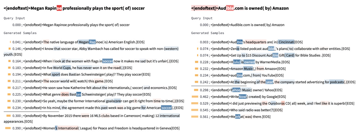
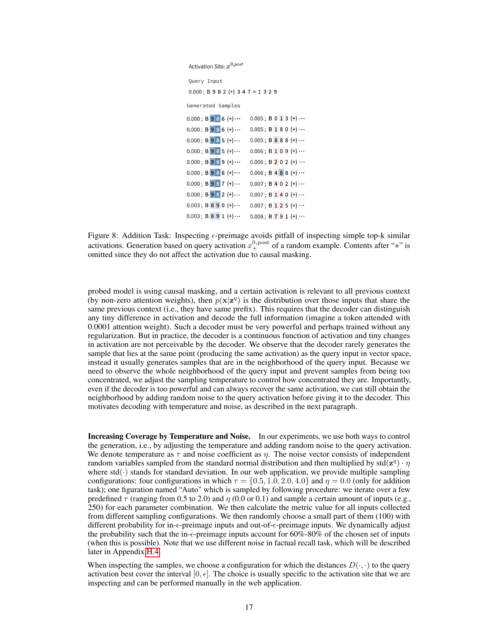
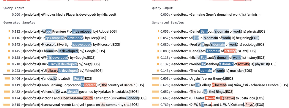
🔼 This figure shows two examples of relation-agnostic retrieval using InversionView. The left panel demonstrates that the activation for the attribute ‘soccer’ is not strictly dependent on the specific relation used in the input, as the attribute remains present even when the relation changes. The right panel illustrates how InversionView identifies information about ‘audio-related’ content regardless of the actual relation in the query input.
read the caption
Figure 41: Examples showing relation-agnostic retrieval. On the left, the information encoded is 'soccer', which is indeed the requested attribute. However, the first sample shows this is not dependent on the relation, since the 'soccer' is still retrieved when relation is 'speaks language'. On the right, the information “audio-related' is encoded, while the relation in the query input is “owned by”.
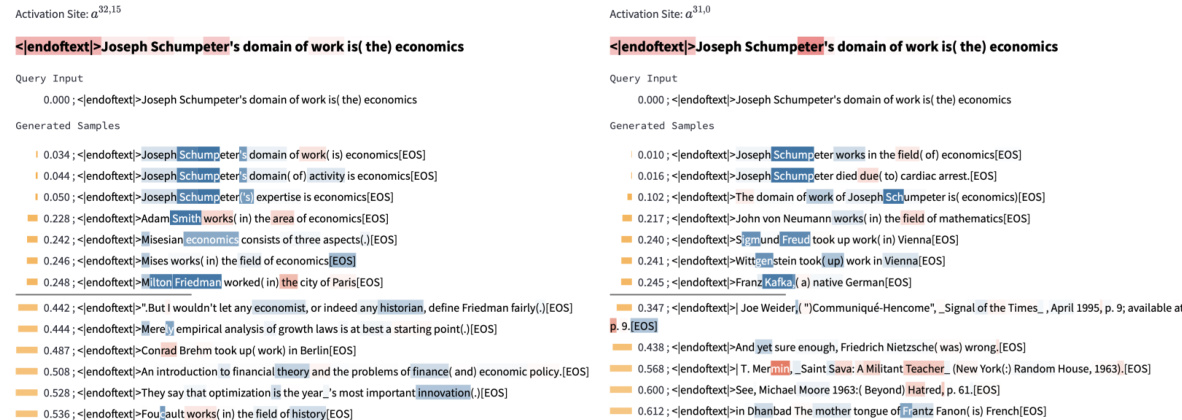
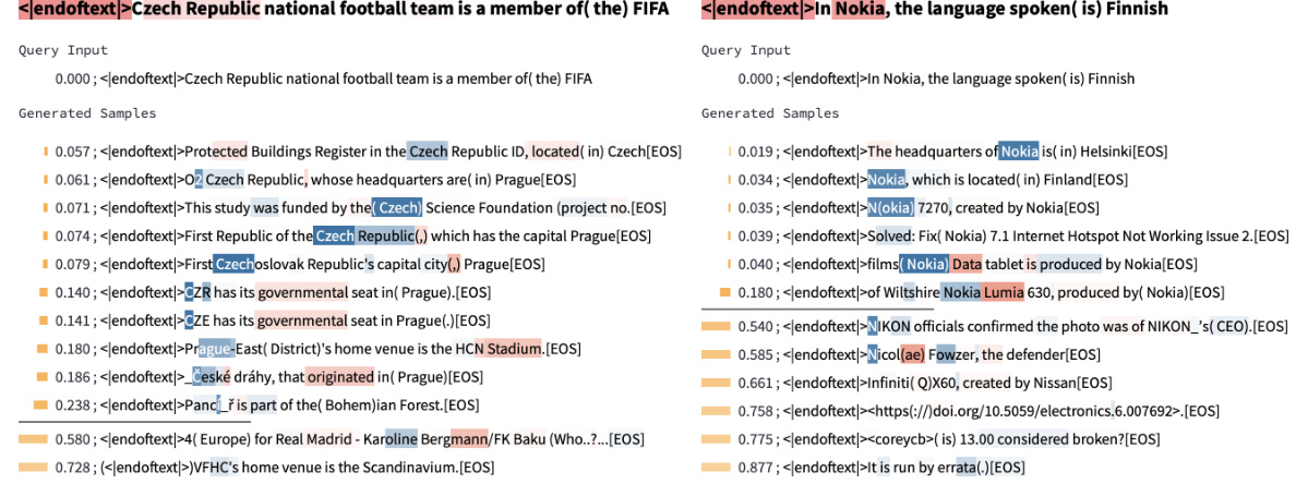
🔼 This figure shows two examples of InversionView applied to different heads. The query input is about Joseph Schumpeter, an Austrian economist. The left panel shows that one head captures information about his profession (’economist’), while the right panel demonstrates a different head capturing information about his language or nationality, relating to Austria. The generated samples highlight that even with the same query input, different activation sites encode different types of information about the subject.
read the caption
Figure 42: Examples showing different attributes of the same subject are extracted by different heads. In the query input, “Joseph Schumpeter” is an Austrian political economist. On the left, the information encoded is “economist”. On the right, the information is about language/nationality (areas around Austria). Again, we emphasize that the facts stated in the sample are not necessarily true.
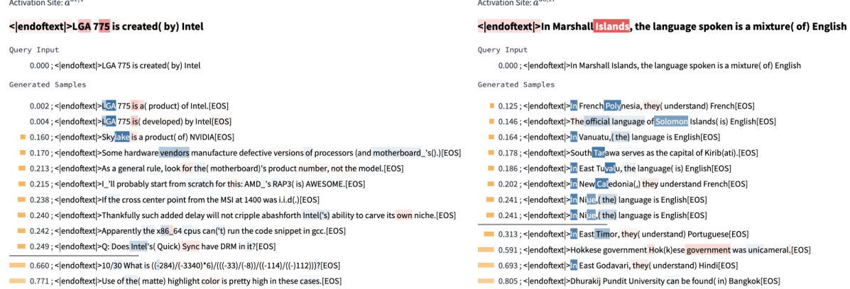
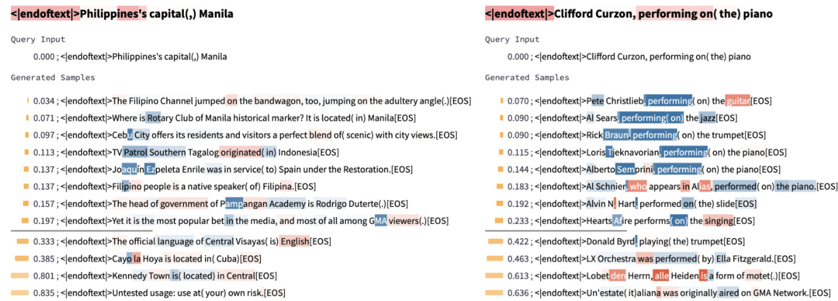
🔼 This figure shows two examples of relation-agnostic retrieval where the information moved by attention heads is not related to the relation in the query input. On the left, the information is about computer hardware. On the right, the information is about island countries. Note that some of the generated statements may not be factually correct.
read the caption
Figure 43: e-preimage showing information about the subject moved by the attention head. On the left, the information is “cpu/computer-hardware-related”. On the right, the information is “island country”. Note that some statements are not correct.

🔼 This figure demonstrates InversionView’s application to a character counting task. It shows how the model processes and retains information about the count of a specific character, even as other information changes. The figure analyzes activations at three different points in the model, comparing distances between activations of samples within and outside the pre-image to reveal how information changes across model layers.
read the caption
Figure 3: InversionView on Character Counting Task. The model counts how often the target character (after '|') occurs in the prefix (before 'l'). B and E denote beginning and end of sequence tokens. The query activation conditions the decoder to generate samples capturing its information content. We show non-cherrypicked samples inside and outside the e-preimage (€ = 0.1) at three activation sites on the same query input. Distance for each sample is calculated between activations corresponding to the parenthesized characters in the query input and the sample. 'True count' indicates the correct count of the target character in the samples (decoder may generate incorrect counts). (a) MLP layer amplifies count information. Comparing the distances before (left) and after (right) the MLP, we see that samples with diverging counts become much more distant from the query activation. (b) In the next layer (':' exclusively attends to target character – copying information from residual stream of target character to the residual stream of ':'), the count is retained but the identity of the target character is no longer encoded ('c', 'm', etc. instead of 'g'), as it is no longer relevant for the predicting the count. Therefore, observing the generations informs us of the activations' content and how it changes across activation sites.

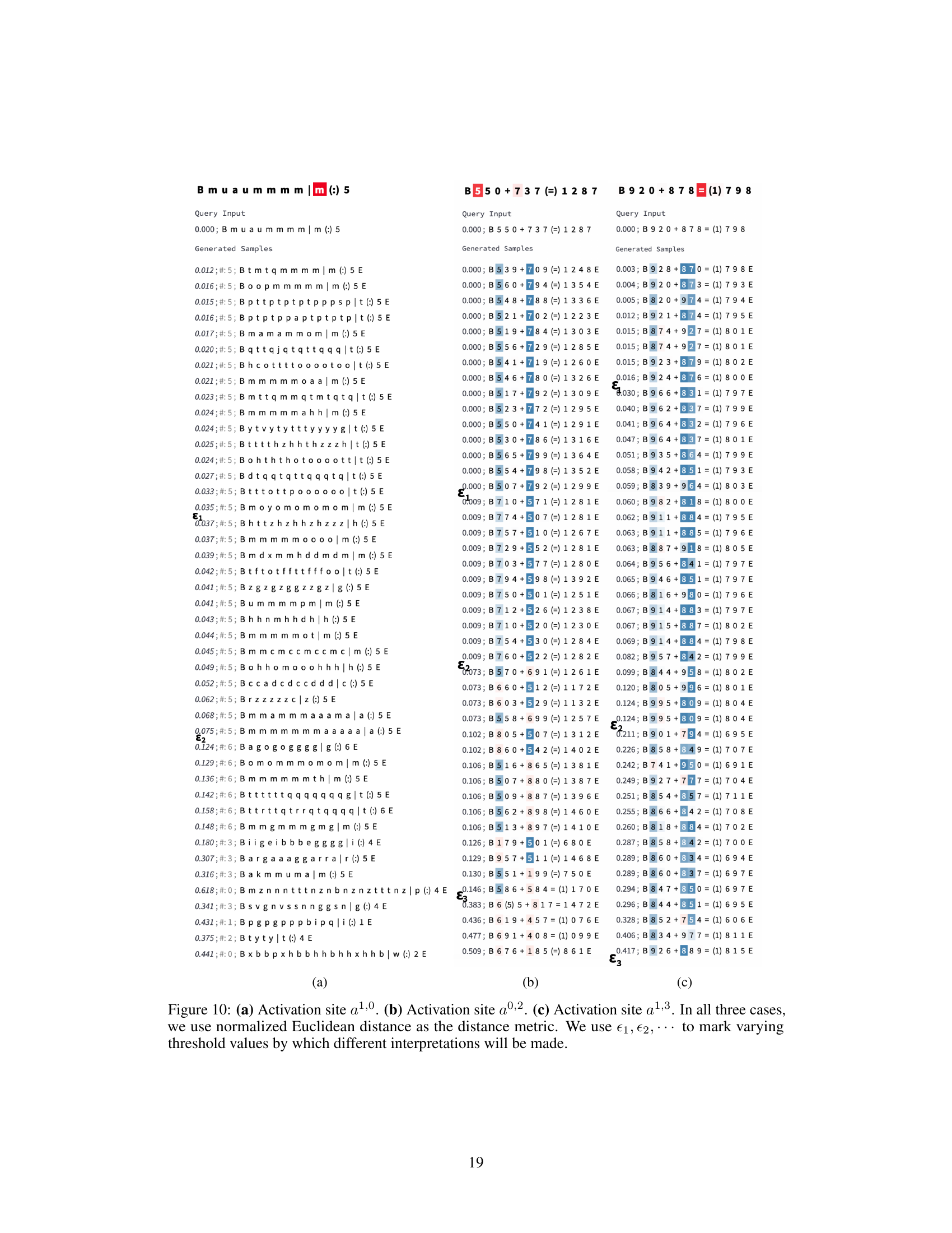
🔼 This figure shows three examples of how different thresholds affect the interpretation of activations in the 3-digit addition task. The x-axis represents the distance between the activation and generated samples, and the y-axis represents the log-probability of the generated sample. Each sub-figure shows three different thresholds (ε1, ε2, ε3), resulting in different interpretations of the encoded information at different activation sites. The different thresholds highlight the tradeoff between sensitivity and completeness of the information obtained from the activation.
read the caption
Figure 10: (a) Activation site a1,0. (b) Activation site a0,2. (c) Activation site a1,3. In all three cases, we use normalized Euclidean distance as the distance metric. We use ε1, ε2, ε3 to mark varying threshold values by which different interpretations will be made.
More on tables
🔼 This table presents the results of applying Direct Logit Attribution (DLA) to the attention heads in the Indirect Object Identification (IOI) circuit. It shows that, except for the first row (Name Mover Head), most heads do not directly connect to the final output in the IOI circuit, and thus DLA cannot effectively decode their information. The table compares the rates at which the expected names appear within the top 30 promoted/suppressed tokens, considering both cases where the name is simply present in the top 30 and when it is the most promoted/suppressed name amongst common and single-token names. The results highlight the limitations of DLA in interpreting model components that indirectly influence the output.
read the caption
Table 4: Applying DLA to the heads in IOI circuit. Except the first row, all heads do not directly connect to final output according to the IOI circuit, the results show DLA cannot decode their information. We do not include those heads in which only position information is encoded. 'Top 30 promoted (suppressed) rate' means the fraction of input examples where the expected name (IO name for the first row, S name for other rows) is inside the top 30 tokens promoted (suppressed) by the head's output. 'Top 30 promoted (suppressed) & 1st name rate' means the expected name is not only inside the top 30 promoted (suppressed) tokens, but also the most promoted (suppressed) name among a list of common and single-token names, so it does not count when another name is ranked higher. Note that a name can be associated with two tokens (with and without a space before it), when calculating the rate, either of them satisfying the condition will count. The rate is calculated over 1000 random IOI examples. As we can see, except for the first row, the expected name is not observable most of the time.

🔼 This table presents the results of an activation patching experiment designed to assess the impact of a specific residual stream (x20,post) on the model’s prediction accuracy in the character counting task. It shows the KL divergence and logit decrement rate for each answer digit (A1, A2, A3, A4/E). These metrics quantify the change in the model’s predictions after patching this residual stream, with smaller values suggesting a minimal effect and therefore indicating this component does not contribute significantly to the result.
read the caption
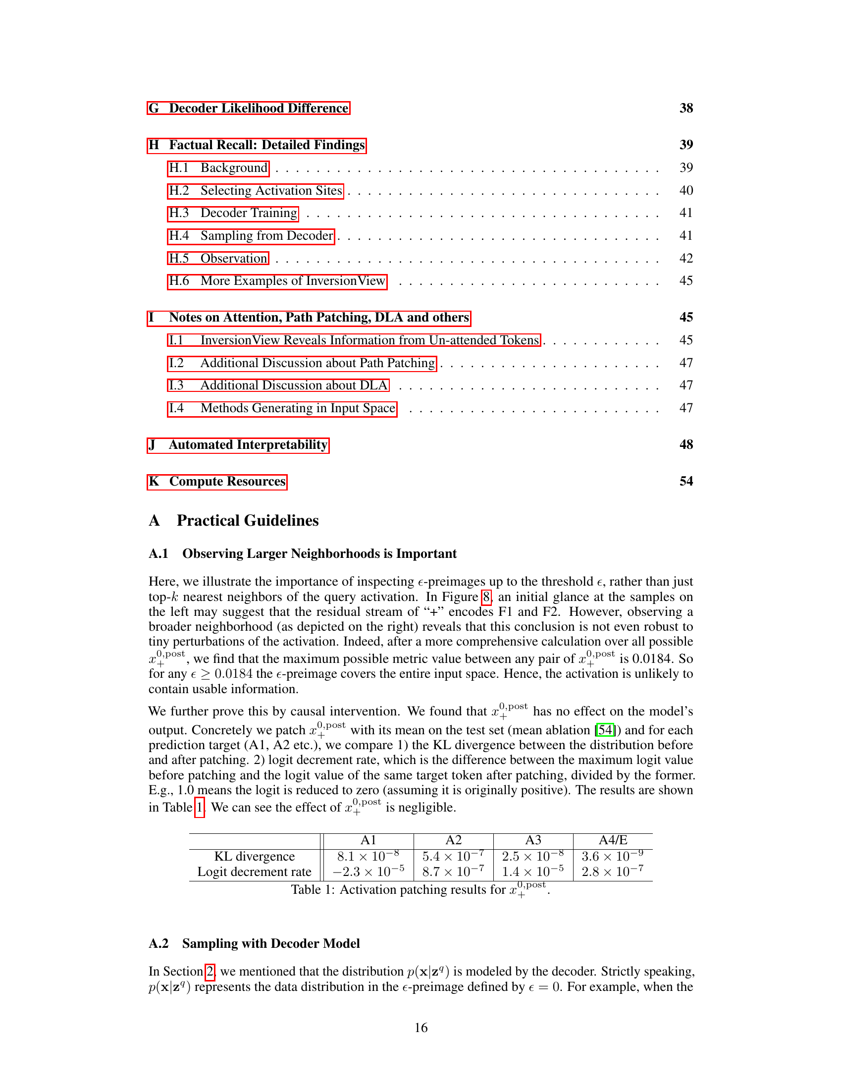
Table 1: Activation patching results for x20,post
🔼 This table presents the results of applying Direct Logit Attribution (DLA) to the attention heads in the Indirect Object Identification (IOI) circuit of a GPT-2 small language model. It evaluates the ability of DLA to identify the indirect object (IO) and subject (S) names by examining the top 30 tokens promoted or suppressed by each attention head’s output. The table demonstrates that except for the first row (Name Mover heads), DLA struggles to reliably identify the expected names within the top 30 tokens, suggesting limitations in using this method for interpreting components not directly influencing the final output.
read the caption
Table 4: Applying DLA to the heads in IOI circuit. Except the first row, all heads do not directly connect to final output according to the IOI circuit, the results show DLA cannot decode their information. We do not include those heads in which only position information is encoded. 'Top 30 promoted (suppressed) rate' means the fraction of input examples where the expected name (IO name for the first row, S name for other rows) is inside the top 30 tokens promoted (suppressed) by the head's output. 'Top 30 promoted (suppressed) & 1st name rate' means the expected name is not only inside the top 30 promoted (suppressed) tokens, but also the most promoted (suppressed) name among a list of common and single-token names, so it does not count when another name is ranked higher. Note that a name can be associated with two tokens (with and without a space before it), when calculating the rate, either of them satisfying the condition will count. The rate is calculated over 1000 random IOI examples. As we can see, except for the first row, the expected name is not observable most of the time.
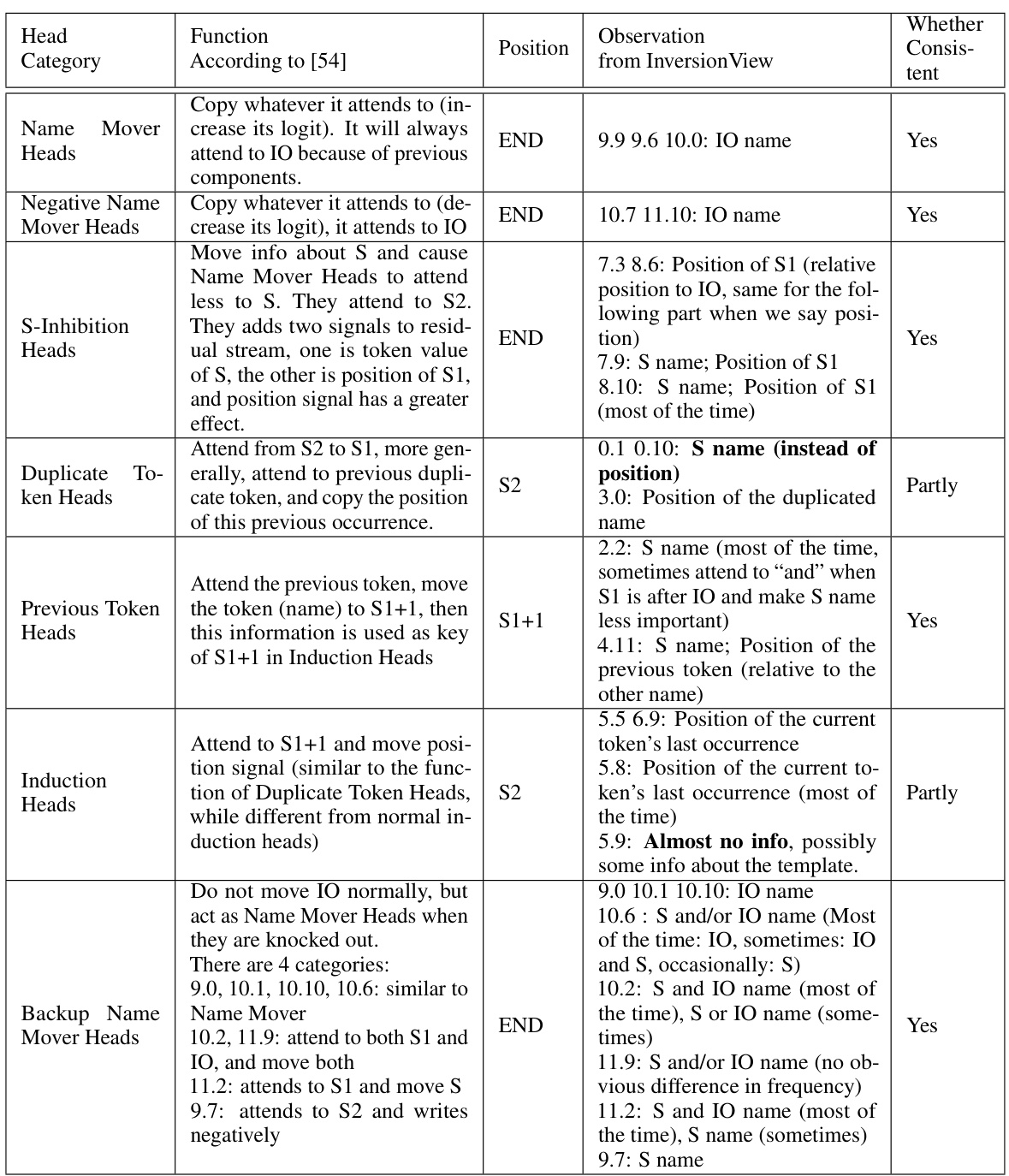
🔼 This table summarizes the comparison of the results from the proposed method and the results from Wang et al. [54]. The first column indicates the category of attention heads, followed by the function of each category according to Wang et al. [54], the position of the query activation, the observation from InversionView, and whether the results are consistent. The information that is different from the original paper is highlighted in bold.
read the caption
Table 2: Column “Position” means the query activation is taken from that position. “S1+1” means the token right after S1. Rows are ordered according to the narration in the original paper. When we say “S name”, it means the the name of S in the query input, but the name is not necessarily S in the samples. This also applies to “IO name”. The information learned by InversionView which is different from the information suggested by Wang et al. [54] is in bold.
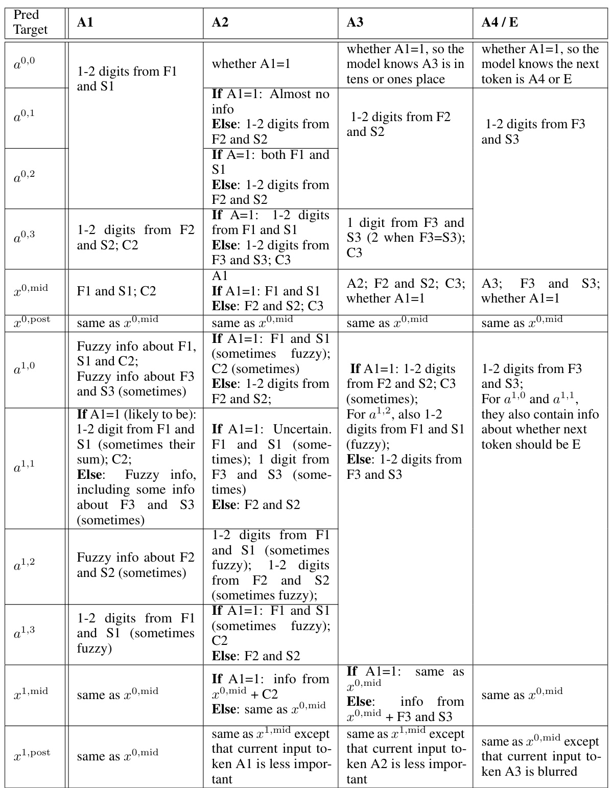
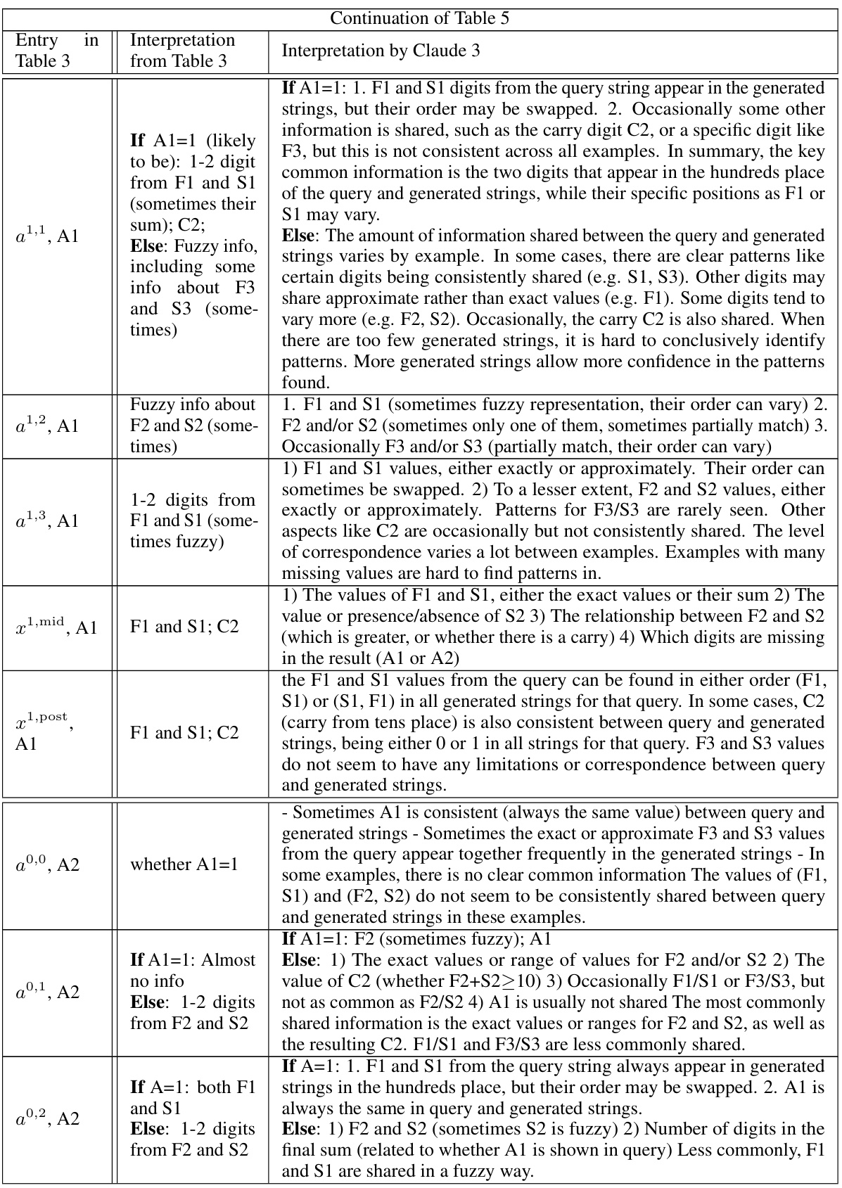
🔼 This table summarizes the findings from the InversionView analysis across different activation sites and positions in the 3-digit addition task. It details what information is encoded at each location (e.g., digits from specific places of the operands, carry bits) and how this information changes across layers (pre, mid, post). The table shows whether the activation’s information content is consistent across different inputs, whether there is a significant difference based on whether the first digit of the answer (A1) is 1 or not, and what other information might be present (e.g., fuzzy information about certain digits).
read the caption
Table 3: Summary of our observations for each activation site and position. “same as” denotes that there is no obvious difference between the two sites for indicated position.

🔼 This table shows the results of applying Direct Logit Attribution (DLA) to the attention heads in the Indirect Object Identification (IOI) circuit of the GPT-2 small model. It demonstrates that for most of the heads (except the first one, which is a Name Mover Head), DLA is unable to decode the expected information. The table compares the success rate of DLA in identifying the expected names (IO or S) within the top 30 promoted or suppressed tokens and also considers the rate when the expected name is the top promoted/suppressed name.
read the caption
Table 4: Applying DLA to the heads in IOI circuit. Except the first row, all heads do not directly connect to final output according to the IOI circuit, the results show DLA cannot decode their information. We do not include those heads in which only position information is encoded. 'Top 30 promoted (suppressed) rate' means the fraction of input examples where the expected name (IO name for the first row, S name for other rows) is inside the top 30 tokens promoted (suppressed) by the head's output. 'Top 30 promoted (suppressed) & 1st name rate' means the expected name is not only inside the top 30 promoted (suppressed) tokens, but also the most promoted (suppressed) name among a list of common and single-token names, so it does not count when another name is ranked higher. Note that a name can be associated with two tokens (with and without a space before it), when calculating the rate, either of them satisfying the condition will count. The rate is calculated over 1000 random IOI examples. As we can see, except for the first row, the expected name is not observable most of the time.

🔼 This table presents the results of applying Direct Logit Attribution (DLA) to the attention heads in the Indirect Object Identification (IOI) circuit from the GPT-2 small model. It shows that except for the first row (Name Mover Heads), the other heads do not have a direct connection to the final output, and thus their information cannot be easily decoded using DLA. The table compares the results of DLA with the findings from InversionView, highlighting the limitations of DLA in deciphering information encoded in model components that don’t directly influence the final prediction. For each head, the table reports the rate of times the expected name (either IO or S, depending on the head) appears in the top 30 tokens that are promoted or suppressed by the head’s output, with and without considering its ranking as the most promoted/suppressed.
read the caption
Table 4: Applying DLA to the heads in IOI circuit. Except the first row, all heads do not directly connect to final output according to the IOI circuit, the results show DLA cannot decode their information. We do not include those heads in which only position information is encoded. 'Top 30 promoted (suppressed) rate' means the fraction of input examples where the expected name (IO name for the first row, S name for other rows) is inside the top 30 tokens promoted (suppressed) by the head's output. 'Top 30 promoted (suppressed) & 1st name rate' means the expected name is not only inside the top 30 promoted (suppressed) tokens, but also the most promoted (suppressed) name among a list of common and single-token names, so it does not count when another name is ranked higher. Note that a name can be associated with two tokens (with and without a space before it), when calculating the rate, either of them satisfying the condition will count. The rate is calculated over 1000 random IOI examples. As we can see, except for the first row, the expected name is not observable most of the time.
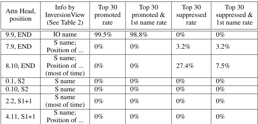
🔼 This table presents the results of applying Direct Logit Attribution (DLA) to the attention heads in the Indirect Object Identification (IOI) circuit from the GPT-2 small model. It compares the results of InversionView with those of DLA, showing that DLA struggles to identify information in heads that do not directly affect the final output. The table indicates the percentage of times the expected name (either the indirect object or subject) appears within the top 30 tokens promoted or suppressed by each attention head, offering insights into how well DLA captures the information contained within specific model components.
read the caption
Table 4: Applying DLA to the heads in IOI circuit. Except the first row, all heads do not directly connect to final output according to the IOI circuit, the results show DLA cannot decode their information. We do not include those heads in which only position information is encoded. 'Top 30 promoted (suppressed) rate' means the fraction of input examples where the expected name (IO name for the first row, S name for other rows) is inside the top 30 tokens promoted (suppressed) by the head's output. 'Top 30 promoted (suppressed) & 1st name rate' means the expected name is not only inside the top 30 promoted (suppressed) tokens, but also the most promoted (suppressed) name among a list of common and single-token names, so it does not count when another name is ranked higher. Note that a name can be associated with two tokens (with and without a space before it), when calculating the rate, either of them satisfying the condition will count. The rate is calculated over 1000 random IOI examples. As we can see, except for the first row, the expected name is not observable most of the time.

🔼 This table presents the results of applying Direct Logit Attribution (DLA) to the attention heads in the Indirect Object Identification (IOI) circuit of a GPT-2 small model. It shows that for most heads, DLA fails to recover the expected name (IO or subject name) within the top 30 tokens, indicating that the information encoded in these attention heads is not directly affecting the model’s output and may be used by other components. The table highlights the limitations of DLA for interpretability in cases where information is indirectly contributing to the final prediction.
read the caption
Table 4: Applying DLA to the heads in IOI circuit. Except the first row, all heads do not directly connect to final output according to the IOI circuit, the results show DLA cannot decode their information. We do not include those heads in which only position information is encoded. 'Top 30 promoted (suppressed) rate' means the fraction of input examples where the expected name (IO name for the first row, S name for other rows) is inside the top 30 tokens promoted (suppressed) by the head's output. 'Top 30 promoted (suppressed) & 1st name rate' means the expected name is not only inside the top 30 promoted (suppressed) tokens, but also the most promoted (suppressed) name among a list of common and single-token names, so it does not count when another name is ranked higher. Note that a name can be associated with two tokens (with and without a space before it), when calculating the rate, either of them satisfying the condition will count. The rate is calculated over 1000 random IOI examples. As we can see, except for the first row, the expected name is not observable most of the time.
🔼 This table presents the results of applying Direct Logit Attribution (DLA) to the attention heads in the Indirect Object Identification (IOI) circuit of a GPT-2 small model. It compares the ability of DLA to identify the expected indirect object (IO) name against the findings from the InversionView method presented in the paper. The table shows that DLA struggles to decode information from most attention heads that don’t directly affect the final output, highlighting a limitation of the DLA approach compared to InversionView.
read the caption
Table 2: Applying DLA to the heads in IOI circuit. Except the first row, all heads do not directly connect to final output according to the IOI circuit, the results show DLA cannot decode their information. We do not include those heads in which only position information is encoded. 'Top 30 promoted (suppressed) rate' means the fraction of input examples where the expected name (IO name for the first row, S name for other rows) is inside the top 30 tokens promoted (suppressed) by the head's output. 'Top 30 promoted (suppressed) & 1st name rate' means the expected name is not only inside the top 30 promoted (suppressed) tokens, but also the most promoted (suppressed) name among a list of common and single-token names, so it does not count when another name is ranked higher. Note that a name can be associated with two tokens (with and without a space before it), when calculating the rate, either of them satisfying the condition will count. The rate is calculated over 1000 random IOI examples. As we can see, except for the first row, the expected name is not observable most of the time.
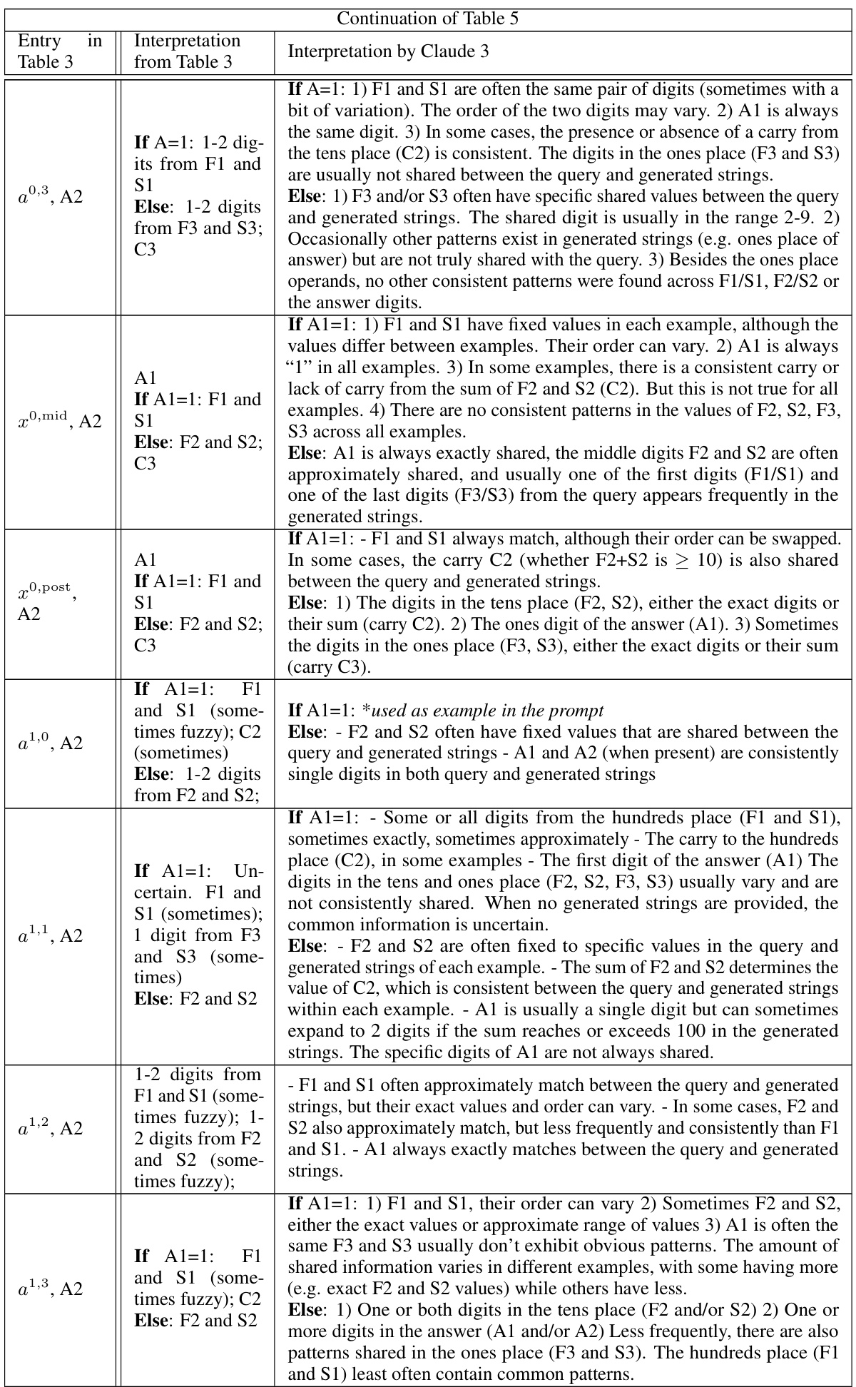
🔼 This table summarizes the qualitative results of applying InversionView to the IOI (Indirect Object Identification) circuit in GPT-2 small. It compares the findings of Wang et al. [54] with those of the current paper, showing the function, observed behavior, position, and consistency of each attention head in the circuit. Key differences in interpretation between the two studies are highlighted in bold.
read the caption
Table 2: Column “Position” means the query activation is taken from that position. “S1+1” means the token right after S1. Rows are ordered according to the narration in the original paper. When we say “S name”, it means the the name of S in the query input, but the name is not necessarily S in the samples. This also applies to “IO name”. The information learned by InversionView which is different from the information suggested by Wang et al. [54] is in bold.

🔼 This table summarizes the findings from the InversionView analysis across different activation sites and positions for a 3-digit addition task. For each activation site and position, it describes what information is present in the activations, whether the information is precise or fuzzy, and how the information changes across layers. The table also notes cases where the information is similar between different sites and positions, indicating consistent representation.
read the caption
Table 3: Summary of our observations for each activation site and position. “same as” denotes that there is no obvious difference between the two sites for indicated position.
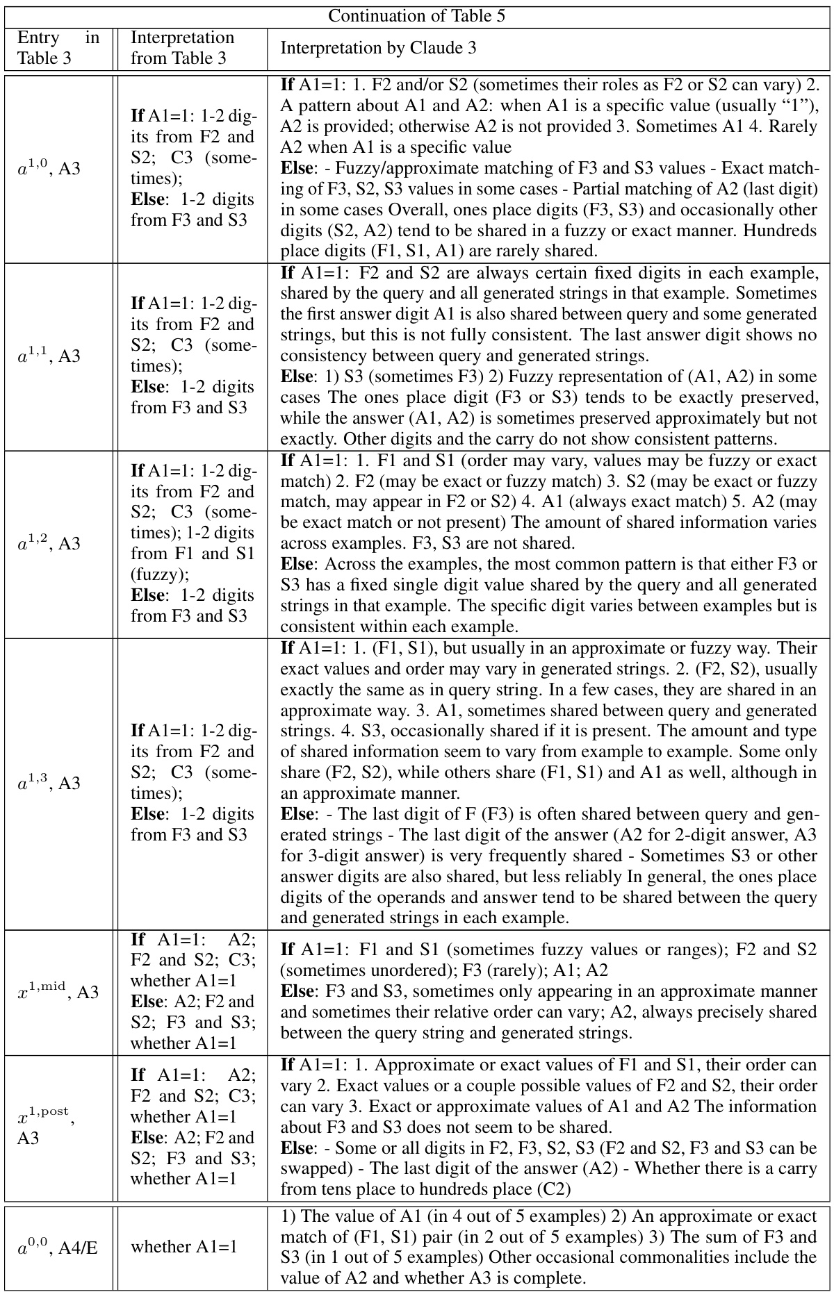
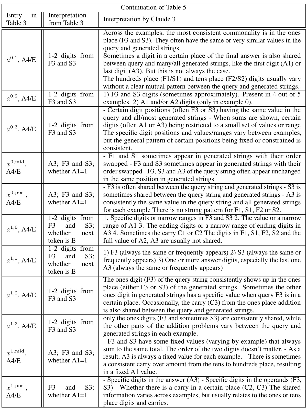
🔼 This table summarizes the information discovered by InversionView for each activation site (e.g., a0,0, a1,0, etc.) and position in the 3-digit addition task. For each activation site and position, it lists the information that is consistently present in the e-preimage (the set of inputs giving rise to similar activations). This information may include specific digits from the operands (F1, F2, F3, S1, S2, S3), carries (C2, C3), and digits in the answer (A1, A2, A3, A4). The table also notes when there are no significant patterns or when the information varies substantially across different inputs.
read the caption
Table 3: Summary of our observations for each activation site and position. “same as” denotes that there is no obvious difference between the two sites for indicated position.
🔼 This table presents the results of applying Direct Logit Attribution (DLA) to various attention heads in the Indirect Object Identification (IOI) circuit within the GPT-2 small model. The table highlights the limitations of DLA in cases where model components do not directly influence the final output. For each attention head, it reports the percentage of times the expected name (IO or subject) appears within the top 30 promoted or suppressed tokens, illustrating the difficulty of accurately interpreting these components using DLA alone.
read the caption
Table 4: Applying DLA to the heads in IOI circuit. Except the first row, all heads do not directly connect to final output according to the IOI circuit, the results show DLA cannot decode their information. We do not include those heads in which only position information is encoded. 'Top 30 promoted (suppressed) rate' means the fraction of input examples where the expected name (IO name for the first row, S name for other rows) is inside the top 30 tokens promoted (suppressed) by the head's output. 'Top 30 promoted (suppressed) & 1st name rate' means the expected name is not only inside the top 30 promoted (suppressed) tokens, but also the most promoted (suppressed) name among a list of common and single-token names, so it does not count when another name is ranked higher. Note that a name can be associated with two tokens (with and without a space before it), when calculating the rate, either of them satisfying the condition will count. The rate is calculated over 1000 random IOI examples. As we can see, except for the first row, the expected name is not observable most of the time.
Full paper#
