TL;DR#
Multivariate time series forecasting is crucial but challenging due to complex temporal and spatial dynamics. Existing models often struggle to capture dynamic spatial correlations accurately, resulting in high variance and limited interpretability. They typically rely on a two-stage process: learning dynamic representations, then generating spatial structures; this is sensitive to small time windows and produces high variance.
This paper introduces Sumba, a novel forecasting model addressing these challenges. Sumba directly parameterizes spatial structures using a learnable matrix basis and a convex combination, enabling effective learning of dynamic spatial structures. Structured parameterization and regularization enhance efficiency and reduce complexity. The model’s well-constrained output space results in lower variance, improved expressiveness, and interpretable dynamics through its coefficient ‘a’.
Key Takeaways#
Why does it matter?#
This paper is important because it proposes a novel forecasting model that significantly improves accuracy and offers interpretable dynamics, addressing limitations of existing methods. It introduces a structured matrix basis to learn dynamic spatial structures, reducing variance and enhancing model expressiveness. This opens avenues for future research in interpretable time series forecasting and dynamic graph learning.
Visual Insights#

🔼 Figure 1(a) shows the overall architecture of the proposed forecasting model, Sumba, which consists of multiple blocks. Each block comprises a Multi-Scale TCN module and a Dynamic GCN module. The Multi-Scale TCN module processes the input data to capture temporal dependencies, while the Dynamic GCN module focuses on generating dynamic spatial structures and fusing spatial information across different series. The final output of the model is the prediction. Figure 1(b) details the inner workings of the Dynamic GCN module. It takes the output from the previous layer and generates the dynamic spatial structure using a structured matrix basis and a matching mechanism. Then, this dynamic graph structure is employed for graph convolutional operations to integrate spatial information before generating the output for the current block.
read the caption
Figure 1: (a) The framework of our proposed Sumba. (b) the detailed structure of the Dynamic GCN module.
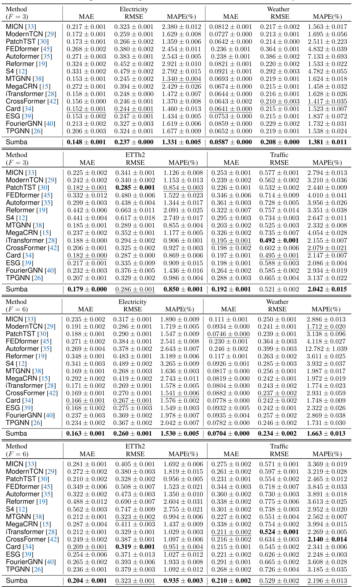
🔼 This table presents the forecasting results for prediction horizons of 3 and 6 time steps on six benchmark datasets (Electricity, Weather, ETTh2, Traffic, PEMS, and Solar-Energy). The results are compared across 15 different forecasting methods, including several transformer-based, TCN-based, and graph neural network based methods. The table shows MAE, RMSE, and MAPE values for each method and dataset, allowing for a comparison of forecasting performance under different conditions.
read the caption
Table 1: The forecasting results with prediction horizons of 3 and 6 on Electricity, Weather, etc.
In-depth insights#
Dynamic Spatial Modeling#
Dynamic spatial modeling in multivariate time series forecasting addresses the limitation of static spatial relationships by acknowledging the evolving nature of correlations between different time series. Traditional methods often assume fixed relationships, which can hinder accuracy, particularly when dealing with real-world data that exhibits changing patterns over time. Dynamic spatial modeling seeks to capture these evolving connections, often through techniques that learn adaptive graph structures or weight matrices. This adaptive approach allows the model to respond to variations in spatial dependencies that may arise due to external factors, temporal patterns, or other dynamic processes. The key challenge lies in effectively learning these dynamic structures, often requiring sophisticated algorithms and sufficient data to handle the added complexity. The resulting models aim to improve forecasting accuracy and provide a more realistic representation of the underlying data generating process.
Structured Matrix Basis#
The concept of a “Structured Matrix Basis” in the context of multivariate time series forecasting suggests a novel approach to modeling dynamic spatial correlations. Instead of using a two-stage process (learning dynamic representations and then spatial structures), this method directly parameterizes the spatial structure generation function using a learnable matrix basis. This basis is structured to enhance efficiency and reduce complexity, resulting in lower variance and easier training. The structured parameterization, possibly involving techniques like SVD, and the use of structure regularization are key innovations. By imposing constraints on the basis matrices, the model gains a degree of interpretability, allowing for insights into the underlying dynamics. The choice of a convex combination of basis matrices to generate the spatial structures ensures a well-constrained output space, further contributing to lower variance. The combination of structured parameterization, regularization, and constrained output space is crucial for effectively capturing the temporal evolution of spatial relationships in multivariate time series, leading to more accurate forecasting.
Interpretable Forecasting#
Interpretable forecasting is a crucial area within time series analysis, aiming to enhance transparency and trust in prediction models. Current approaches often prioritize accuracy over explainability, creating a “black box” effect where understanding the model’s decision-making process is difficult. This limits the ability to debug models, identify potential biases, and build user confidence. Interpretable methods, however, strive to provide insights into the underlying relationships and patterns driving the predictions. This could involve techniques that highlight feature importance, visualize the model’s decision boundaries, or provide simple, human-understandable rules. The value of interpretability is multifaceted; it allows for better model validation, facilitating the identification of errors and biases; it increases user trust and acceptance of the model’s predictions; and it enables domain experts to gain meaningful insights from the model’s output. Despite its importance, achieving high accuracy alongside full interpretability remains a challenge. Future research should focus on developing novel methods that effectively balance these competing goals, and address the trade-off between model accuracy and the level of interpretability achieved.
Ablation Study Analysis#
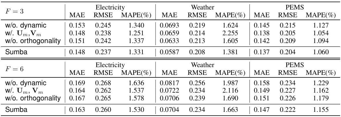
An ablation study systematically removes components of a model to assess their individual contributions. In the context of a time series forecasting model, this might involve removing elements like the dynamic spatial structure generation function, the structured matrix parameterization, or the orthogonality constraint. By observing the impact on forecasting accuracy after each ablation, researchers can quantify the importance of each component. A well-designed ablation study should isolate each component’s effect, revealing which features are crucial for achieving high performance and which might be redundant or detrimental. Furthermore, analyzing the ablation results helps determine the model’s robustness and its sensitivity to various factors. The insights gained through this analysis are invaluable for improving the model, enhancing its interpretability, and ultimately leading to a more effective and efficient forecasting system. The ablation study can also highlight areas for future research, suggesting which aspects of the model design warrant further refinement or exploration.
Future Research#
Future research directions stemming from this structured matrix basis model for multivariate time series forecasting could explore several key areas. Improving the adaptive mechanism for the dynamic spatial structure generation function is crucial, potentially leveraging more sophisticated attention mechanisms or graph neural networks to capture complex, evolving relationships between time series. Investigating alternative parameterizations beyond the proposed structured matrix basis could lead to more efficient and expressive models. This might involve exploring low-rank approximations, sparse matrix techniques, or other factorizations. Another promising avenue would be developing robust methods for handling missing data or noise, which commonly affect real-world multivariate time series. The interpretability of the model, a significant strength, could be further enhanced by developing techniques for visualizing and interpreting the learned dynamic spatial structures in a more intuitive way. Finally, extending the model to handle different types of time series data (e.g., irregularly sampled, high-dimensional) and applying it to a broader range of applications would greatly increase its practical impact.
More visual insights#
More on figures

🔼 This figure visualizes the change in the weight of the matrix basis coefficient ‘a’ over a week for both the Solar-Energy and Electricity datasets. The heatmaps show that most weights are concentrated on two basis matrices (matrix 1 and matrix 4), suggesting the existence of two dominant spatial structures. These structures alternate regularly, corresponding to day and night for Solar-Energy data (as expected), and showing a midnight-specific correlation in the Electricity dataset.
read the caption
Figure 2: The change of a over one week.

🔼 This figure visualizes the changes in the coefficient ‘a’ over a week for the Electricity and Solar-Energy datasets. The x-axis represents time (hourly), and the y-axis represents the index of five basis matrices (1-5). The color intensity indicates the weight of each coefficient ‘a’ at a given time and matrix index. The heatmaps show the evolution of the dominant spatial structures for each dataset across time. The observed alternating patterns (Solar-Energy) correspond to day/night cycles of the solar power generation and its spatial correlations.
read the caption
Figure 2: The change of a over one week.

🔼 This figure shows the training curves of several time series forecasting methods on the Electricity and Weather datasets. The prediction length (F) is set to 3. The plot shows the MAE (Mean Absolute Error) for each method over the training epochs. It illustrates the convergence speed of the different models. Sumba, ModernTCN, and ESG show fast convergence within 5 epochs, while other methods (Card, FourierGNN, TPGNN) require more epochs to converge.
read the caption
Figure 7: The training curves on Electricity and Weather datasets with prediction length F = 3.

🔼 The figure shows the sensitivity analysis of the dimension of basis M on the performance of the proposed model. The x-axis represents different values of M (from 1 to 10), and the y-axis represents MAE, RMSE, and MAPE for Electricity, Weather, ETTh2, Traffic, Solar, and PEMS datasets. The boxplots show the performance variation across different datasets and values of M. The results suggest that an optimal value of M exists for each dataset, improving model performance significantly when M > 1.
read the caption
Figure 3: The sensitivity of the dimension of basis M.

🔼 This figure shows the sensitivity analysis of the proposed Sumba model to the hyperparameter H, representing the history window size. The plots display the performance (MAE, RMSE, and MAPE) across six benchmark datasets (Electricity, Weather, PEMS, ETTh2, Solar, and Traffic) with varying H values (24, 48, 96, 168). The results illustrate how changes in the history window size affect the model’s accuracy in forecasting.
read the caption
Figure 6: The sensitivity of our method to the history window H.

🔼 This figure shows the training curves for the first 10 epochs on the Electricity and Weather datasets. It compares the convergence speed of Sumba against several other time series forecasting methods, including ModernTCN, Card, ESG, FourierGNN, and TPGNN. The figure highlights that Sumba, ModernTCN, and ESG exhibit rapid convergence within 5 epochs, whereas other methods require more epochs to reach convergence.
read the caption
Figure 7: The training curves on Electricity and Weather datasets with prediction length F = 3.
More on tables
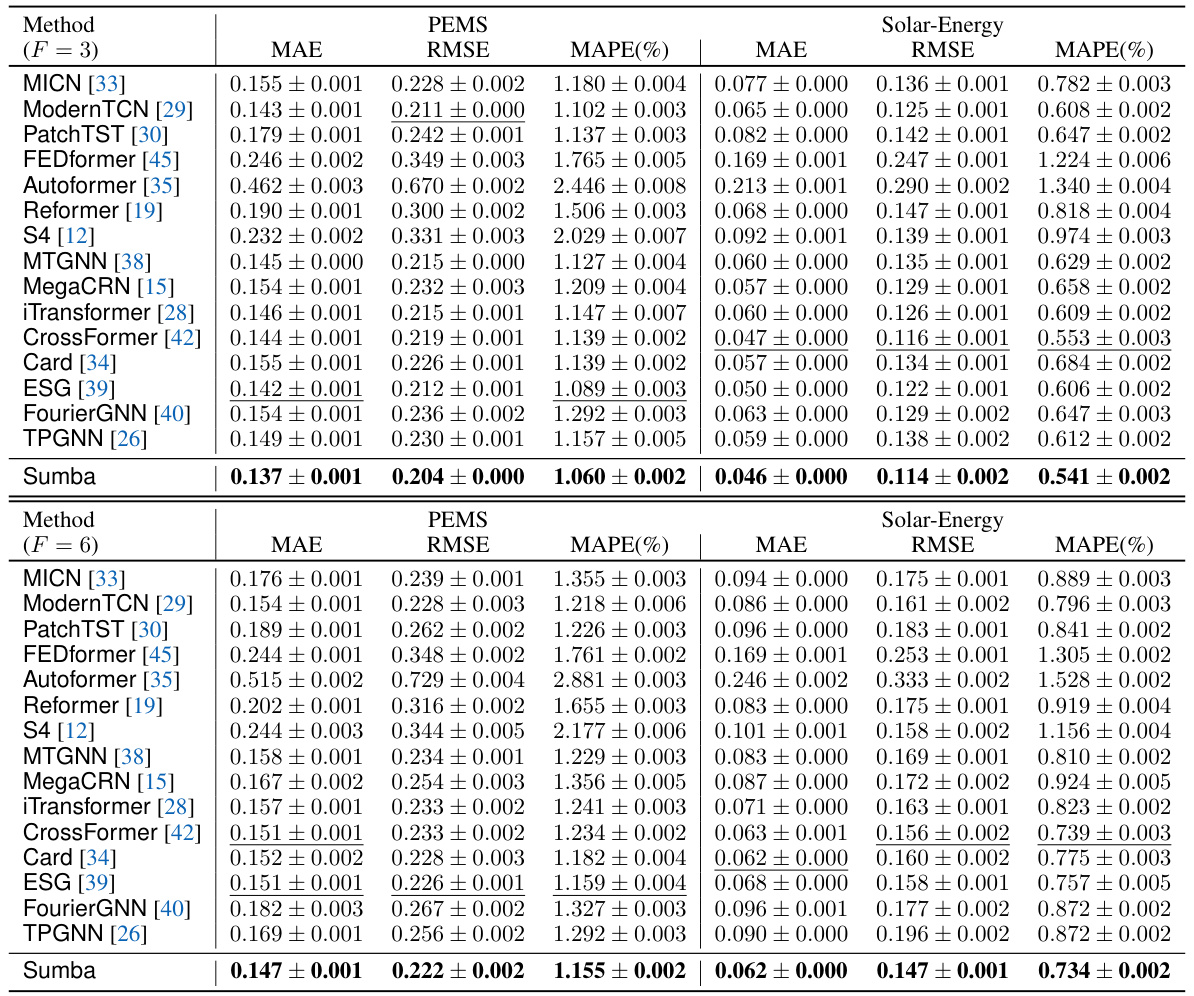
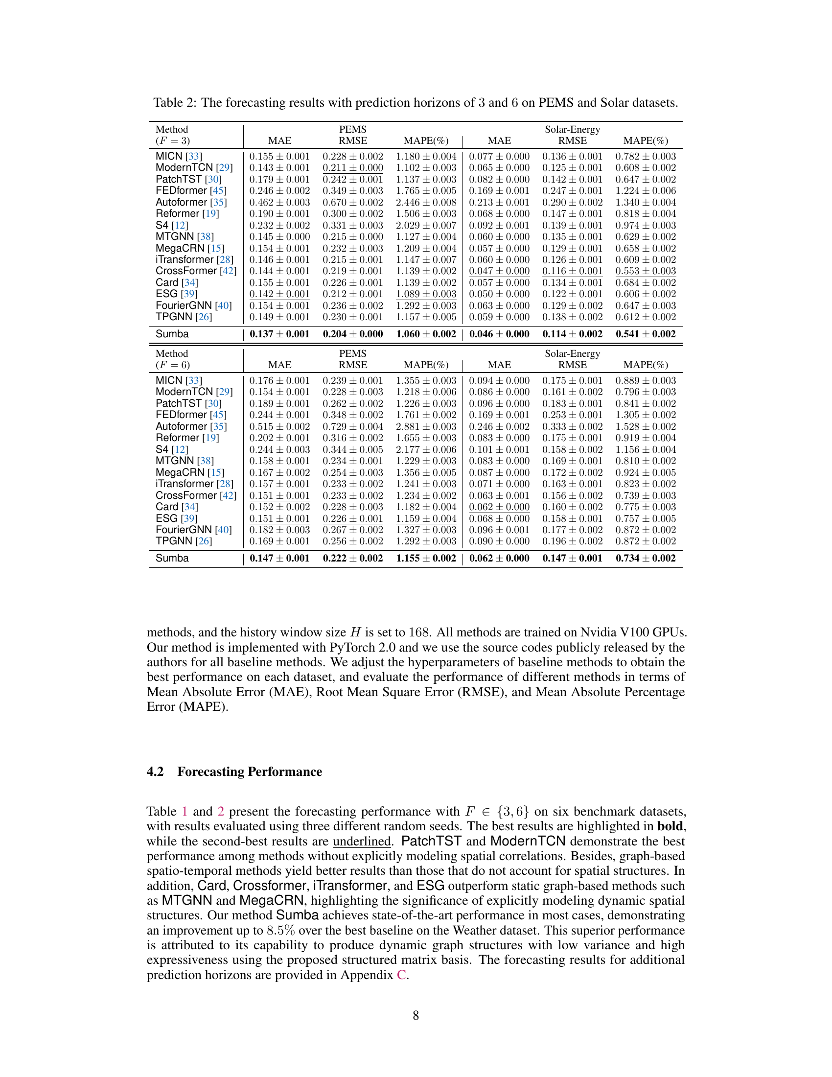
🔼 This table presents the forecasting results obtained using various prediction horizons (3 and 6) on two benchmark datasets: PEMS (traffic data) and Solar-Energy (solar power production data). The table compares the performance of the proposed Sumba model against several baseline forecasting methods across different evaluation metrics: MAE (Mean Absolute Error), RMSE (Root Mean Squared Error), and MAPE (Mean Absolute Percentage Error). The results are shown for both short-term (F=3) and medium-term (F=6) predictions.
read the caption
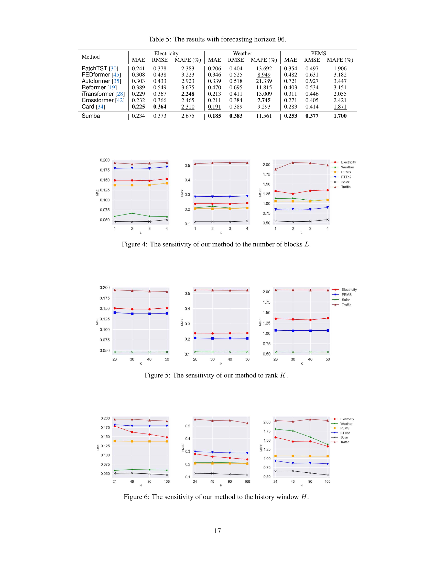
Table 2: The forecasting results with prediction horizons of 3 and 6 on PEMS and Solar datasets.
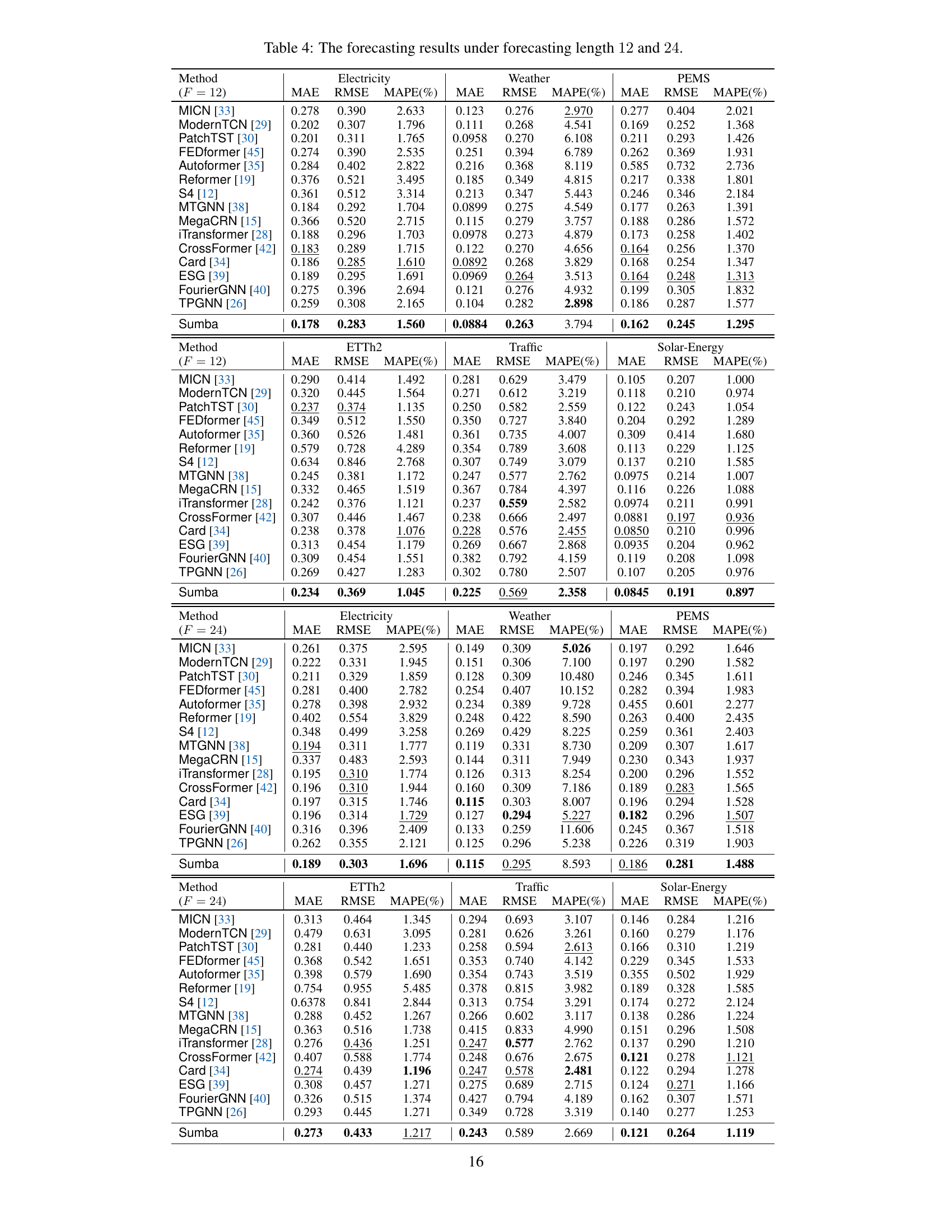
🔼 This table presents the forecasting results of the proposed Sumba model and 15 other baseline methods on six benchmark datasets (Electricity, Weather, ETTh2, Traffic, PEMS, and Solar-Energy) for prediction horizons of 3 and 6 time steps. The evaluation metrics used are MAE (Mean Absolute Error), RMSE (Root Mean Square Error), and MAPE (Mean Absolute Percentage Error). The table allows for a comparison of the performance of Sumba against various existing time series forecasting techniques, highlighting its effectiveness in different datasets and prediction lengths.
read the caption
Table 1: The forecasting results with prediction horizons of 3 and 6 on Electricity, Weather, etc.
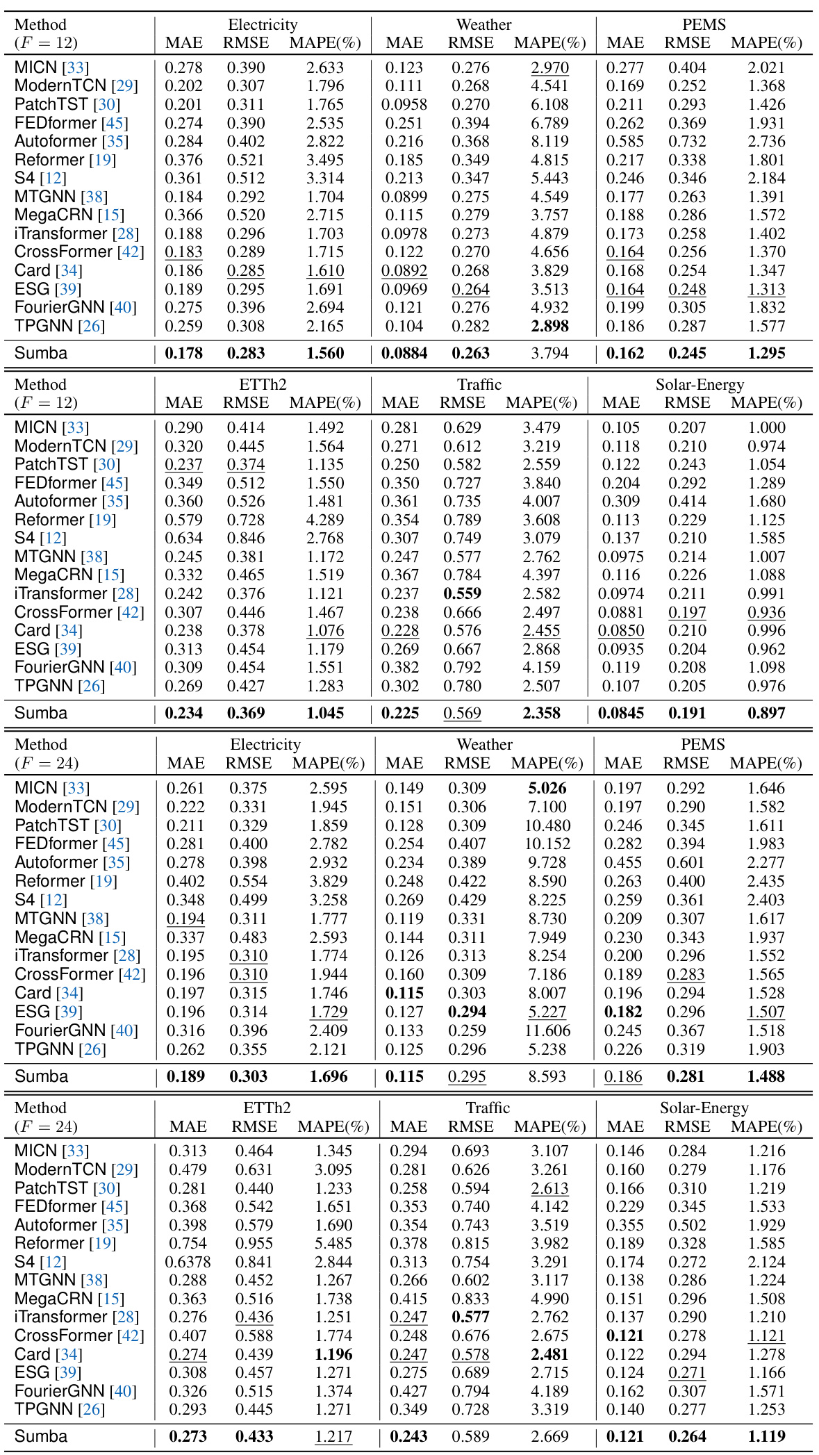
🔼 This table presents the forecasting results of the proposed Sumba model and 15 benchmark models on six datasets (Electricity, Weather, ETTh2, Traffic, PEMS, and Solar-Energy) using two prediction horizons (F=3 and F=6). The evaluation metrics used are MAE (Mean Absolute Error), RMSE (Root Mean Squared Error), and MAPE (Mean Absolute Percentage Error). The table allows for comparison of the performance of Sumba against other state-of-the-art models in multivariate time series forecasting across different datasets and forecasting lengths.
read the caption
Table 1: The forecasting results with prediction horizons of 3 and 6 on Electricity, Weather, etc.

🔼 This table presents the forecasting results achieved by Sumba and 15 other benchmark methods across six datasets (Electricity, Weather, ETTh2, Traffic, PEMS, and Solar-Energy) for prediction horizons of 3 and 6 time steps. The results are evaluated using three metrics: Mean Absolute Error (MAE), Root Mean Square Error (RMSE), and Mean Absolute Percentage Error (MAPE). The table allows for a comparison of Sumba’s performance against various state-of-the-art forecasting methods.
read the caption
Table 1: The forecasting results with prediction horizons of 3 and 6 on Electricity, Weather, etc.
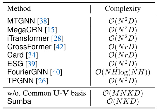
🔼 This table compares the computational complexity of different time series forecasting methods. The complexity is expressed using Big O notation, with N representing the number of nodes, M the dimension of the matrix basis, D the dimension of the node embedding or hidden representation, r < N, and K « N. The table shows that methods such as MTGNN, MegaCRN, iTransformer, ESG, and TPGNN have a complexity of O(N2D) due to using inner products of node embeddings. CrossFormer and Card reduce the complexity to O(NrD) by employing router mechanisms and summarized tokens. FourierGNN’s complexity is O(NHlog(NH)) because of the construction of hypervariable graphs. Sumba, with its low-rank approximation and common coordinate transformations, achieves a complexity of O(NKD), making it more computationally efficient, especially for large N.
read the caption
Table 6: The complexity of different methods.
Full paper#
