TL;DR#
Bayesian inference often assumes a known prior distribution for optimal estimation in inverse problems. However, in practice, priors are usually unknown. Algorithm unrolling offers a deep learning-based solution by training neural networks to mimic iterative inference algorithms. Despite empirical success, theoretical guarantees for this approach remained elusive.
This research addresses this gap by focusing on compressed sensing, proving that unrolled AMP networks, trained using layerwise gradient descent, converge to the same denoisers used in Bayes AMP and thus achieve near-optimal mean squared error. The study also demonstrates the method’s robustness to general priors, low dimensionality, and non-Gaussian settings, showing superior performance to Bayes AMP in several cases.
Key Takeaways#
Why does it matter?#
This paper is crucial because it provides the first rigorous proof that unrolled networks can match the performance of optimal Bayesian methods. This bridges the gap between the empirical success of algorithm unrolling and theoretical understanding, opening new avenues for research in deep learning for Bayesian inference and related fields.
Visual Insights#
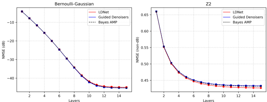
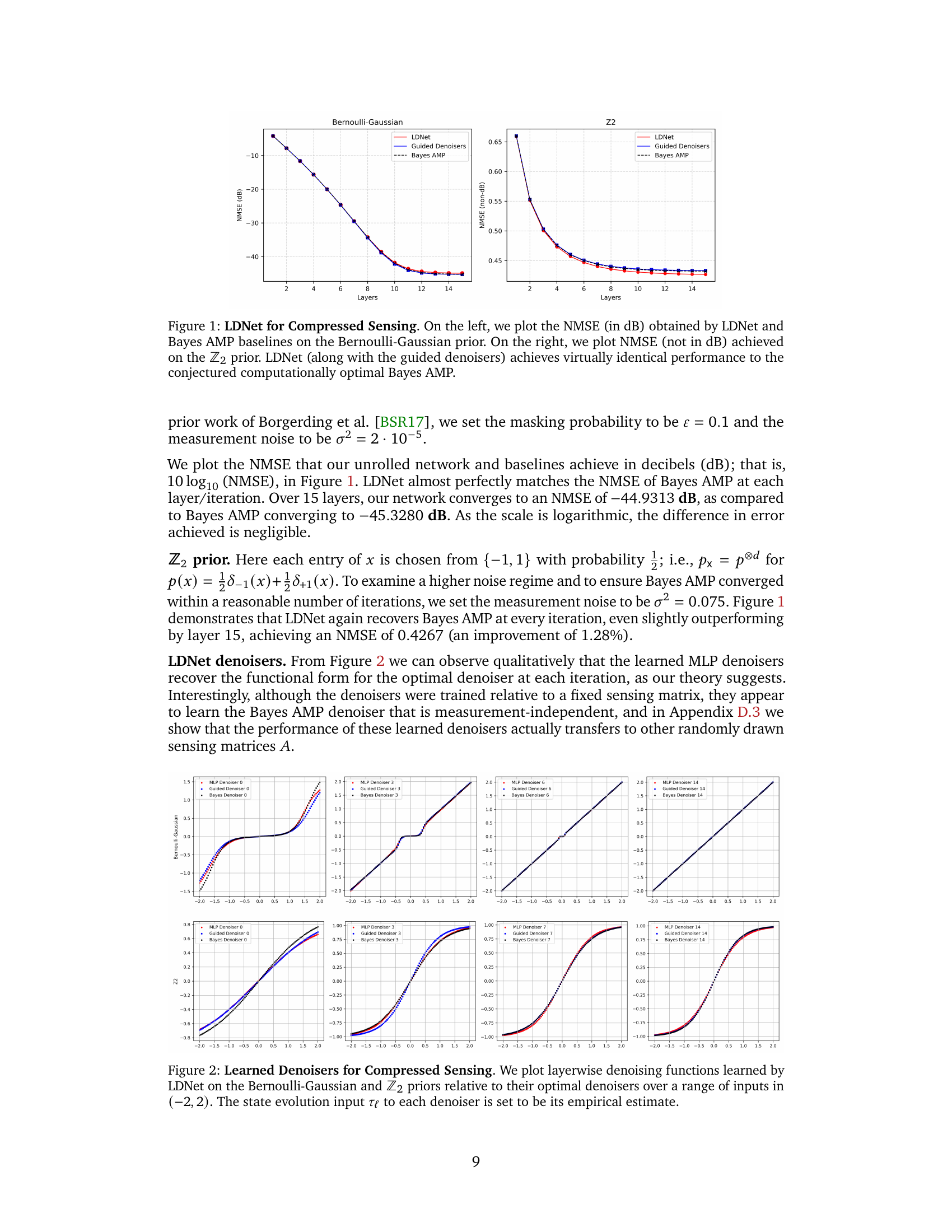
🔼 This figure compares the Normalized Mean Squared Error (NMSE) achieved by three different methods for compressed sensing: LDNet (Learned Denoising Network), guided denoisers, and Bayes AMP (Approximate Message Passing). Two different priors are used: Bernoulli-Gaussian and Z2. The left panel shows the NMSE in dB for the Bernoulli-Gaussian prior, while the right panel shows NMSE (not in dB) for the Z2 prior. The results demonstrate that LDNet and guided denoisers achieve nearly identical performance to the theoretically optimal Bayes AMP, showcasing the effectiveness of the unrolled network architecture in learning the optimal denoising functions.
read the caption
Figure 1: LDNet for Compressed Sensing. On the left, we plot the NMSE (in dB) obtained by LDNet and Bayes AMP baselines on the Bernoulli-Gaussian prior. On the right, we plot NMSE (not in dB) achieved on the Z2 prior. LDNet (along with the guided denoisers) achieves virtually identical performance to the conjectured computationally optimal Bayes AMP.

🔼 This figure compares the Normalized Mean Squared Error (NMSE) achieved by the proposed LDNet model and two baseline models (Bayes AMP and guided denoisers) for two different signal priors in compressed sensing experiments. The left panel shows the NMSE (in decibels) for a Bernoulli-Gaussian prior, and the right panel shows NMSE (not in dB) for a Z2 prior. The results demonstrate that the LDNet achieves performance nearly identical to Bayes AMP, which is conjectured to be optimal. The plot includes the NMSE as a function of the number of layers used in each method.
read the caption
Figure 1: LDNet for Compressed Sensing. On the left, we plot the NMSE (in dB) obtained by LDNet and Bayes AMP baselines on the Bernoulli-Gaussian prior. On the right, we plot NMSE (not in dB) achieved on the Z2 prior. LDNet (along with the guided denoisers) achieves virtually identical performance to the conjectured computationally optimal Bayes AMP.
In-depth insights#
Unrolled AMP#
The concept of “Unrolled AMP” combines the strengths of approximate message passing (AMP) algorithms with the flexibility of neural networks. AMP algorithms provide a theoretically grounded approach to solving inverse problems, particularly in compressed sensing, offering strong optimality guarantees under specific conditions. However, AMP’s reliance on knowing the true prior distribution limits its practical applicability. Unrolling involves constructing a neural network whose layers mimic the iterative steps of an AMP algorithm. This allows the network to learn optimal denoisers and adapt to unknown priors, overcoming the limitations of traditional AMP. The training process, often employing layer-wise techniques, further enhances performance. Theoretical analysis of unrolled AMP aims to bridge the gap between empirical success and rigorous guarantees, proving that under certain conditions the network converges to the performance of optimal Bayesian AMP. This approach offers a powerful, potentially more robust and adaptable, alternative to traditional AMP, especially in low-dimensional or non-standard settings.
Bayes AMP#
Bayes AMP, or Bayesian Approximate Message Passing, is a powerful algorithm for solving inverse problems. It leverages the principles of Bayesian inference by incorporating prior knowledge about the signal being estimated. This prior knowledge helps to regularize the solution and improve accuracy, especially in high-dimensional or ill-conditioned settings. Unlike traditional methods that rely solely on the observed data, Bayes AMP incorporates probabilistic information about the signal, making it more robust to noise and uncertainty. While theoretically optimal under certain assumptions, Bayes AMP’s computational complexity can be high, and its implementation can be challenging, particularly in situations where the prior distribution is unknown or complex. This motivates the development of methods, such as unrolling neural networks, which can learn to approximate Bayes AMP’s behavior without explicit knowledge of the prior. This is a key idea explored in the research paper, demonstrating that unrolled networks can, under certain conditions, provably achieve the same performance as Bayes AMP but with improved practicality. Therefore, the concept of Bayes AMP stands as a crucial theoretical benchmark in signal processing and machine learning research, guiding the development of more efficient and practical inference methods.
LDNet Training#
The training of LDNet, a learned denoising network unrolling approximate message passing (AMP), is a crucial aspect of its performance. Instead of end-to-end training, which often leads to suboptimal solutions, the authors employ a layerwise training strategy. This approach iteratively trains each layer’s denoising function (MLP) by minimizing the mean squared error (MSE) of its layer-specific estimate, while freezing the weights of previously trained layers. This layerwise method, coupled with initializing each layer’s weights using the previous layer’s learned denoiser and optional further finetuning, proves essential for escaping suboptimal local minima and achieving performance comparable to Bayes AMP. The layerwise training’s efficacy stems from the inherent iterative structure of AMP, where each step builds upon the previous one. By training layer by layer, the network effectively learns the optimal denoising functions for each AMP iteration. This technique offers a practical method to learn Bayes-optimal denoisers without explicitly knowing the data’s prior distribution, enabling the network to adapt to diverse signal priors and overcoming the limitations of traditional AMP implementations.
Theoretical Guarantees#
The research paper focuses on establishing rigorous theoretical guarantees for the performance of unrolled denoising networks in solving inverse problems. The core argument centers on proving that these networks, when trained appropriately, can achieve performance comparable to Bayes-optimal methods, even without explicit knowledge of the underlying data distribution. This is a significant advance because Bayes-optimal methods often rely on unrealistic assumptions about the prior. The theoretical analysis leverages a combination of state evolution and neural tangent kernel (NTK) techniques, which offer a powerful framework for understanding the training dynamics and generalization capabilities of neural networks. The results show that under specific conditions (smooth, sub-Gaussian priors), the unrolled network’s denoisers converge to those of Bayes AMP, ensuring near-optimal performance. However, the theoretical guarantees are currently limited to specific prior distributions and settings. Future work could potentially relax these assumptions and broaden the scope of the theoretical results to encompass more general scenarios, making the findings more widely applicable. The successful combination of state evolution and NTK analysis offers a promising avenue for future research, opening up potential to analyze and improve other unrolled algorithms in the context of Bayesian inference.
Future Research#
Future research directions stemming from this work could explore extending the theoretical guarantees to non-product priors and more general settings beyond compressed sensing and rank-one matrix estimation. The current limitations of the theory regarding product priors necessitate investigating methods to handle the complexities of non-product distributions. Another important area is developing a more comprehensive understanding of the interplay between the architecture of the unrolled network and the efficiency of learning. Exploring different network architectures and training strategies, including potentially non-layerwise methods, might lead to improvements in both learning speed and performance. Finally, rigorous theoretical analysis of the learned denoisers and their relationship to optimal Bayes AMP is crucial. This would involve a deeper investigation of the learned functions’ properties and their approximation to optimal denoisers, which could offer significant insights into the practical capabilities and limitations of algorithm unrolling.
More visual insights#
More on figures
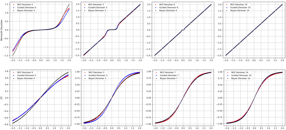
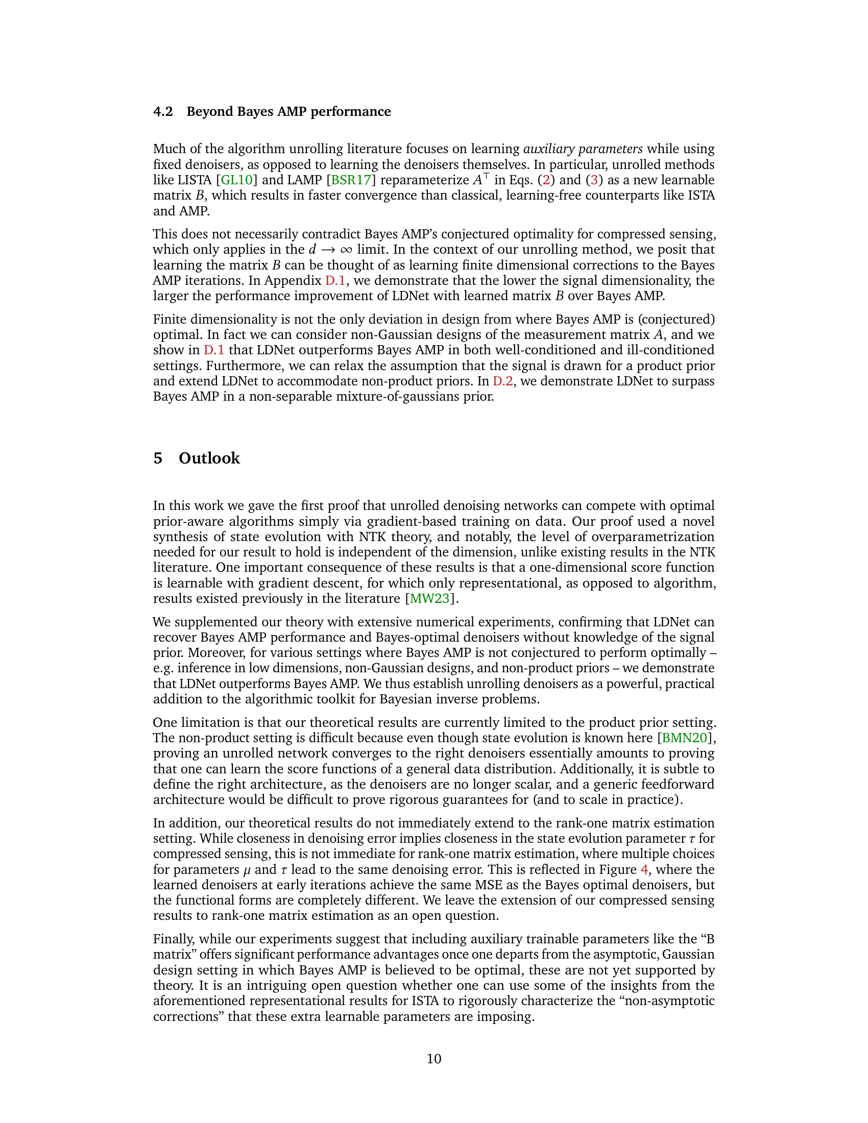
🔼 This figure compares the denoising functions learned by the LDNet model with the theoretically optimal denoisers for both Bernoulli-Gaussian and Z2 priors in a compressed sensing task. It visualizes how well the learned denoisers approximate the optimal denoisers at different layers (iterations) of the unrolled network. The x-axis represents the input to the denoiser, and the y-axis represents the denoiser’s output. Different colors represent different layers of the network and the optimal denoiser.
read the caption
Figure 2: Learned Denoisers for Compressed Sensing. We plot layerwise denoising functions learned by LDNet on the Bernoulli-Gaussian and Z2 priors relative to their optimal denoisers over a range of inputs in (−2, 2). The state evolution input τe to each denoiser is set to be its empirical estimate.
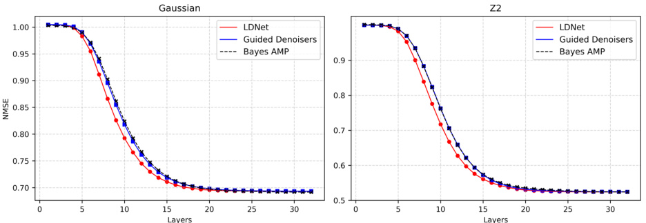
🔼 This figure compares the performance of LDNet and Bayes AMP on two different priors (Bernoulli-Gaussian and Z2) for compressed sensing. The left panel shows NMSE in dB for the Bernoulli-Gaussian prior, while the right panel shows NMSE (not in dB) for the Z2 prior. The results demonstrate that LDNet achieves nearly identical performance to Bayes AMP, which is considered computationally optimal. The results also include a comparison with guided denoisers.
read the caption
Figure 1: LDNet for Compressed Sensing. On the left, we plot the NMSE (in dB) obtained by LDNet and Bayes AMP baselines on the Bernoulli-Gaussian prior. On the right, we plot NMSE (not in dB) achieved on the Z2 prior. LDNet (along with the guided denoisers) achieves virtually identical performance to the conjectured computationally optimal Bayes AMP.

🔼 This figure compares the learned denoising functions from the LDNet model with the optimal denoising functions (from Bayes AMP) for different layers (0,3,6,14) and two different prior distributions (Bernoulli-Gaussian and Z2). The x-axis represents the input to the denoiser, and the y-axis represents the output. The plot shows that the LDNet successfully learns denoising functions that closely approximate the optimal functions, especially as the number of layers increases. The empirical estimate of the state evolution parameter, τe, is used for each denoiser.
read the caption
Figure 2: Learned Denoisers for Compressed Sensing. We plot layerwise denoising functions learned by LDNet on the Bernoulli-Gaussian and Z2 priors relative to their optimal denoisers over a range of inputs in (−2, 2). The state evolution input τe to each denoiser is set to be its empirical estimate.

🔼 This figure shows the results of experiments where the dimension m of the measurement matrix A is varied while keeping the ratio of the dimension of the measurement matrix to the signal dimension constant. The NMSE (dB) is plotted as a function of the number of layers in the network. The figure shows that the performance gap between the proposed learned B method and Bayes AMP increases as the dimension m decreases. This suggests that the improvement offered by learning the auxiliary parameter B becomes more pronounced in lower-dimensional settings.
read the caption
Figure 5: Learned B with Decreasing Dimension. We hold δ = ½ fixed while scaling m from 200 down to 100. Plots show NMSE (dB) performance of unrolling denoisers and learning B vs. Bayes AMP for randomly drawn measurement matrices. There is an increasing gap in performance as m decreases.

🔼 This figure compares the performance of LDNet (with a learnable parameter B) against several baselines (Bayes AMP, ISTA, and CoSaMP) for compressed sensing with non-Gaussian measurement matrices. The two subfigures show results for two different types of matrices: a truncated random orthogonal matrix and a truncated random Gram matrix. The results indicate that LDNet achieves lower normalized mean squared error (NMSE) and converges faster than the other methods in both scenarios.
read the caption
Figure 6: Non-Gaussian Measurements. On the left, we plot LDNet with learnable B compared to several baselines for a random truncated orthogonal measurement matrix, and on the right, for a random truncated Gram matrix. LDNet outperforms the other baselines in NMSE as well as convergence.

🔼 This figure shows the performance of the proposed method (LDNet with learnable matrix B) compared to Bayes AMP in low-dimensional settings. Three different dimensions (m = 100, 150, 200) are shown, with the y-axis representing NMSE (dB) and x-axis representing the number of layers. As the dimension decreases, the performance gap between LDNet and Bayes AMP increases, indicating that LDNet with a learnable matrix B is advantageous in low-dimensional regimes where Bayes AMP’s asymptotic optimality does not apply.
read the caption
Figure 5: Learned B with Decreasing Dimension. We hold δ = ½ fixed while scaling m from 200 down to 100. Plots show NMSE (dB) performance of unrolling denoisers and learning B vs. Bayes AMP for randomly drawn measurement matrices. There is an increasing gap in performance as m decreases.

🔼 This figure compares the performance of the proposed LDNet and Bayes AMP on rank-one matrix estimation for two different non-product priors: Z2 and a mixture of Gaussians. The plot shows the NMSE (normalized mean squared error) versus the number of layers in the network. The results demonstrate that the LDNet significantly outperforms Bayes AMP in both cases, achieving lower NMSE with fewer layers.
read the caption
Figure 7: Multi-Dimensional LDNet for Rank-One Matrix Estimation. On the left, we plot the NMSE obtained by LDNet and Bayes AMP on Z2, while the right plots are on the mixture of Gaussians. LDNet outperforms Bayes AMP by significant margins.
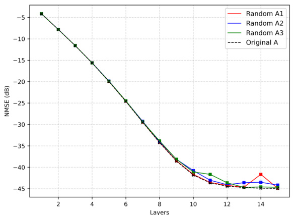
🔼 This figure shows the robustness of the learned denoisers to different sensing matrices. The NMSE (dB) is plotted against the number of layers for four different scenarios: the original sensing matrix used during training, and three other randomly generated Gaussian sensing matrices. The results demonstrate that the learned denoisers generalize well to new sensing matrices, indicating that the learning process is not highly dependent on the specific sensing matrix used during training.
read the caption
Figure 8: Transfer Experiments. Above we plot the NMSE (in dB) over 15 iterations for different choices of measurement matrices coupled with our learned MLP denoisers, including the training-time sensing matrix. We see that the denoising functions are roughly transferable to several random Gaussian measurement settings, suggesting the learning process is not coupled to the fixed sensing matrix seen during training.
Full paper#
