TL;DR#
Diffusion Transformers (DiTs) are powerful generative models but suffer from slow training. Existing training strategies often lack consistency across different datasets. Furthermore, the effectiveness of supervision at specific training steps is limited. This paper addresses these issues by proposing a novel way to assess the robustness of training strategies using Signal-to-Noise Ratio (SNR) probability density functions.
To tackle the issues, FasterDiT proposes a unified accelerating strategy based on experimental results and the proposed SNR analysis. This strategy includes a new supervision method, which improves the efficiency of the training process. These contributions lead to a significant speedup in training time (7x faster) while maintaining comparable performance to existing state-of-the-art models. The approach focuses on simplicity and practicality, emphasizing easy implementation and broad applicability.
Key Takeaways#
Why does it matter?#
This paper is crucial for researchers in diffusion models due to its significant speedup in training time without architectural changes. It offers a novel perspective on training efficiency and robustness, leading to improvements in existing models and opening new avenues for optimizing the training of other generative models. The focus on simple and practical design strategies makes its findings broadly applicable, impacting the efficiency of large-scale training.
Visual Insights#
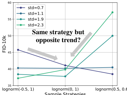
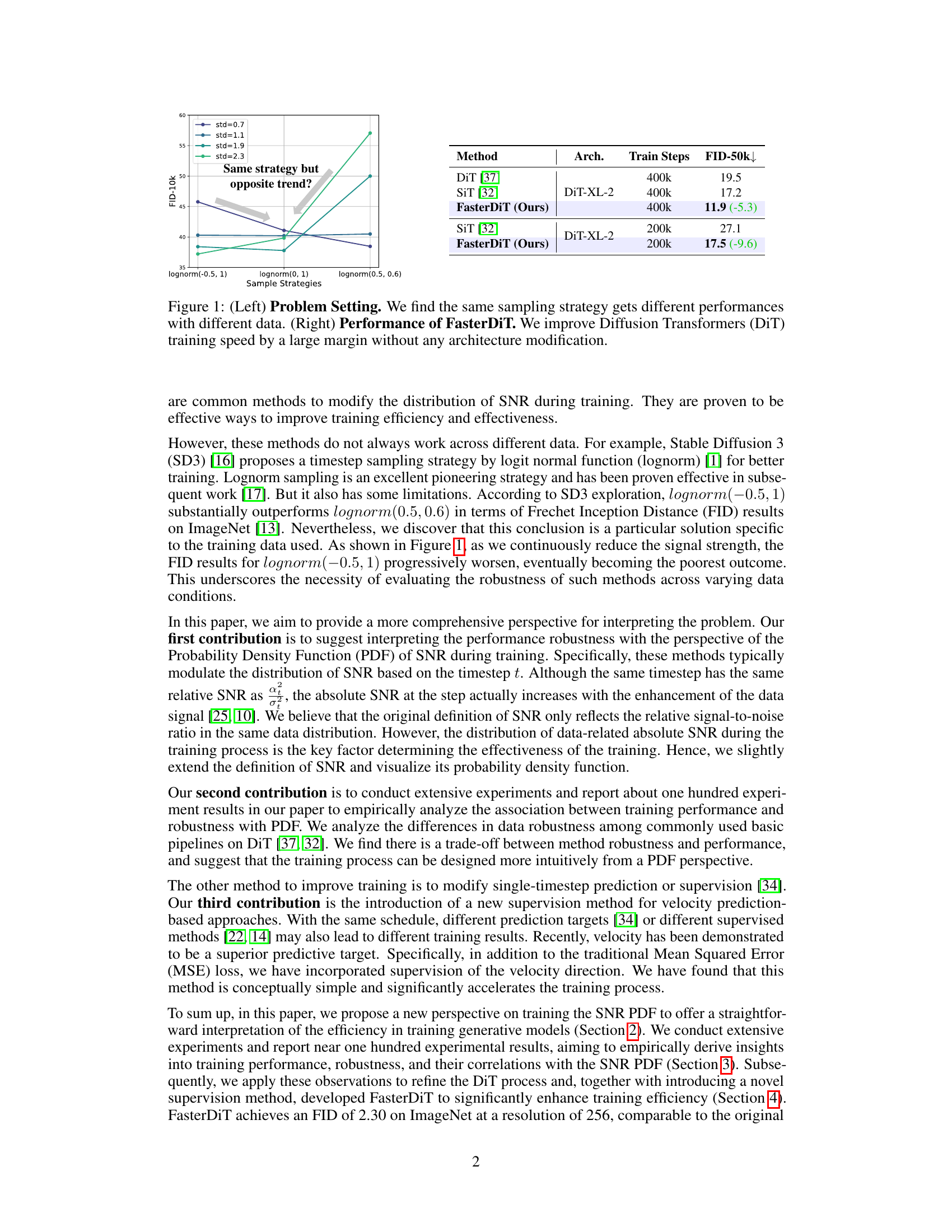
🔼 The left panel shows that using the same sampling strategy (different lognormal distributions) leads to significantly different performance results depending on the dataset used. This highlights the lack of robustness in existing strategies for diffusion model training. The right panel demonstrates the improvement achieved by FasterDiT, showcasing a substantial reduction in FID (Frechet Inception Distance) for various sampling strategies while using fewer training steps, effectively accelerating the training process significantly.
read the caption
Figure 1: (Left) Problem Setting. We find the same sampling strategy gets different performances with different data. (Right) Performance of FasterDiT. We improve Diffusion Transformers (DiT) training speed by a large margin without any architecture modification.
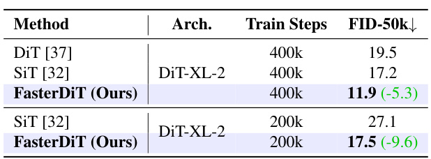
🔼 This figure shows a comparison of the performance of different methods for training diffusion transformers. The left side shows that the same sampling strategy can have different performances depending on the data. The right side shows that the proposed method, FasterDiT, significantly improves the training speed of diffusion transformers without any architectural modifications.
read the caption
Figure 1: (Left) Problem Setting. We find the same sampling strategy gets different performances with different data. (Right) Performance of FasterDiT. We improve Diffusion Transformers (DiT) training speed by a large margin without any architecture modification.
In-depth insights#
DiT Training Issues#
Diffusion Transformers (DiT), while powerful, suffer from slow convergence, hindering their practical application. This slow training is attributed to two main issues. First, existing training strategies, such as noise scheduling and loss weighting, lack consistency across different datasets. What works well for one dataset might not generalize to others. Second, the effectiveness of supervision at specific timesteps is limited, meaning that the model doesn’t learn equally well from all points in the denoising process. These issues highlight a need for improved training strategies that are more robust and efficient, achieving faster convergence without requiring architectural modifications.
SNR PDF Analysis#
The SNR PDF analysis section likely explores the probability distribution of the signal-to-noise ratio (SNR) at different training stages. This is a novel approach because it moves beyond simply analyzing the average SNR, which may mask crucial information. By examining the SNR’s distribution, researchers can identify where the training process focuses most of its attention. This might reveal if the training spends excessive time in low-SNR or high-SNR regions, which could indicate inefficiencies. The PDF analysis may also help to explain why certain training strategies work well with some datasets but not others—the robustness of a strategy is reflected in the stability of its SNR PDF across various data. The shape of the SNR PDF may be used to guide the design of more effective training strategies, leading to accelerated convergence and improved model performance. In essence, this analysis is a powerful diagnostic tool for understanding and improving the efficiency of diffusion model training.
FasterDiT Strategy#
The FasterDiT strategy focuses on accelerating Diffusion Transformer (DiT) training without architectural changes. Its core innovation lies in a novel interpretation of the Signal-to-Noise Ratio (SNR), suggesting that observing the Probability Density Function (PDF) of the SNR across different data intensities offers crucial insights into training robustness and efficiency. The method empirically demonstrates that a well-focused SNR-PDF, neither too narrow nor too broad, leads to faster and more robust training. FasterDiT leverages this insight by subtly modifying the training data’s standard deviation, thus shifting the SNR-PDF’s focus to the optimal region identified through experiments. A supplementary velocity prediction supervision method further enhances training speed, improving upon traditional noise-only supervision. The strategy’s simplicity and effectiveness are highlighted by achieving results comparable to DiT but with significantly faster training times, demonstrating its potential for broad application in large-scale generative modeling.
High-Res Results#
A dedicated ‘High-Res Results’ section would be crucial for evaluating the model’s performance on higher-resolution images. It would ideally showcase image generation quality at resolutions beyond those used in the main training and validation experiments, demonstrating the model’s ability to generalize. Key metrics such as FID (Fréchet Inception Distance) and IS (Inception Score) should be reported for these high-resolution outputs. Qualitative assessments, including a diverse selection of generated images, would also add significant value. By examining the results, it will be possible to assess whether the model maintains its quality and coherence when tasked with producing more detailed images. The analysis would also be needed to examine if artifacts, blurriness, or other degradation issues appear at these higher resolutions. Finally, comparing high-resolution results with those from lower resolutions is vital to understanding the model’s scaling behavior and identifying potential bottlenecks.
Future Work#
Future research directions stemming from this work on accelerating Diffusion Transformer training could explore several promising avenues. Extending the proposed FasterDiT methodology to other generative models beyond DiT and SiT is crucial, demonstrating its generalizability and potential impact on a broader range of image generation tasks. Investigating the impact of different data modalities (e.g., video, 3D models) on the effectiveness of FasterDiT’s strategies would offer valuable insights into the technique’s limitations and adaptability. Further research into the theoretical underpinnings of the SNR PDF’s influence on training efficiency is warranted, potentially leading to more sophisticated and robust training strategies. Finally, exploring the scalability of FasterDiT for extremely large-scale training scenarios and higher resolutions would solidify its practical value in real-world applications. Addressing these areas will provide a more complete understanding of the method’s strengths and weaknesses and enhance its impact on the field.
More visual insights#
More on figures

🔼 This figure shows the robustness of four different noise schedules (DDPM-linear, Flow-linear, DDPM-cosine, Flow-cosine) under varying data signal intensities. The x-axis represents the standard deviation (std) of the input data, and the y-axis represents the FID-10k score. Each subplot shows the performance of a particular noise schedule for different standard deviations. The figure demonstrates that the performance of each noise schedule varies significantly depending on the input data’s signal intensity, indicating different levels of robustness. The figure highlights that a single schedule does not consistently perform well across different datasets, indicating a tradeoff between the performance and robustness.
read the caption
Figure 2: Robustness of Different Noise Schedules. By scaling input to different standard deviations, we compare the data robustness of four schedules [22, 35, 29, 32], including diffusion and flow matching. Note that we set the prediction target as noise for a fair comparison. We find that different data signal intensities lead to different generative performances and different schedules have different robustness.

🔼 This figure shows the probability density functions (PDFs) of the signal-to-noise ratio (SNR) for four different noise schedules ([22, 35, 29, 32]) at three different standard deviations (std). The x-axis represents the log-SNR (in dB), and the y-axis represents the density. The different colored lines represent different schedules, and the different lines within each color represent different standard deviations. The figure illustrates how the distribution of SNR changes with different noise schedules and data signal strength. This is used to illustrate how different scheduling strategies affect the training process and robustness across data variations. The gray shaded area is mentioned in the text but not clearly depicted in the figure, making this detail ambiguous.
read the caption
Figure 3: SNR PDF of different noise schedules [22, 35, 29, 32]. The figure illustrates the signal-to-noise ratio (SNR) probability density functions (PDFs) for various schedules and standard deviations (see Section 2).

🔼 This figure shows the impact of using a lognorm distribution for timestep sampling on the performance and robustness of different training schedules. The left panels show the probability density function (PDF) of SNR for linear and lognorm-modified linear training schedules. The right panels show how the FID changes with different standard deviations for these two schedules. It highlights that while using lognorm can improve the upper bound of the performance, it can also decrease the robustness of training to changes in data intensity.
read the caption
Figure 4: Influence of Weghting Dring Training. We use lognorm(0, 1) as Stable Diffusion3 [16]. The essence of this approach is to enhance the local focus of the PDF during the training process. This increases the upper bound of the training, but it also reduces the robustness of the training process to variations in the data.

🔼 This figure compares the robustness of four different noise schedules (DDPM linear, DDPM cosine, Flow linear, Flow cosine) across various signal intensities. The x-axis represents the standard deviation of the input data, scaled to simulate varying signal strengths. The y-axis shows the FID (Fréchet Inception Distance), a metric evaluating the quality of generated images. The results demonstrate that a single noise schedule’s performance fluctuates greatly with changes in input data intensity, and that different noise schedules exhibit varying degrees of robustness across different input intensities.
read the caption
Figure 2: Robustness of Different Noise Schedules. By scaling input to different standard deviations, we compare the data robustness of four schedules [22, 35, 29, 32], including diffusion and flow matching. Note that we set the prediction target as noise for a fair comparison. We find that different data signal intensities lead to different generative performances and different schedules have different robustness.

🔼 This figure shows the effects of modulating the standard deviation of training data on the FID score. The shaded region highlights the optimal standard deviation that shifts the probability density function of the signal-to-noise ratio (SNR) to improve the training efficiency. The graph demonstrates that small modifications to the training process can lead to large improvements in the training performance of the diffusion transformers.
read the caption
Figure 7: Training Details. Our training pipeline involves only minimal modifications to the code.

🔼 This figure compares the robustness of four different noise schedules (DDPM-linear, DDPM-cosine, Flow-linear, Flow-cosine) across varying data signal intensities. The robustness is evaluated by observing changes in FID (Fréchet Inception Distance) score as the standard deviation of the input data is scaled. The results show that different noise schedules exhibit varying levels of robustness, with some performing consistently well across different signal strengths, while others show significant performance fluctuations.
read the caption
Figure 2: Robustness of Different Noise Schedules. By scaling input to different standard deviations, we compare the data robustness of four schedules [22, 35, 29, 32], including diffusion and flow matching. Note that we set the prediction target as noise for a fair comparison. We find that different data signal intensities lead to different generative performances and different schedules have different robustness.

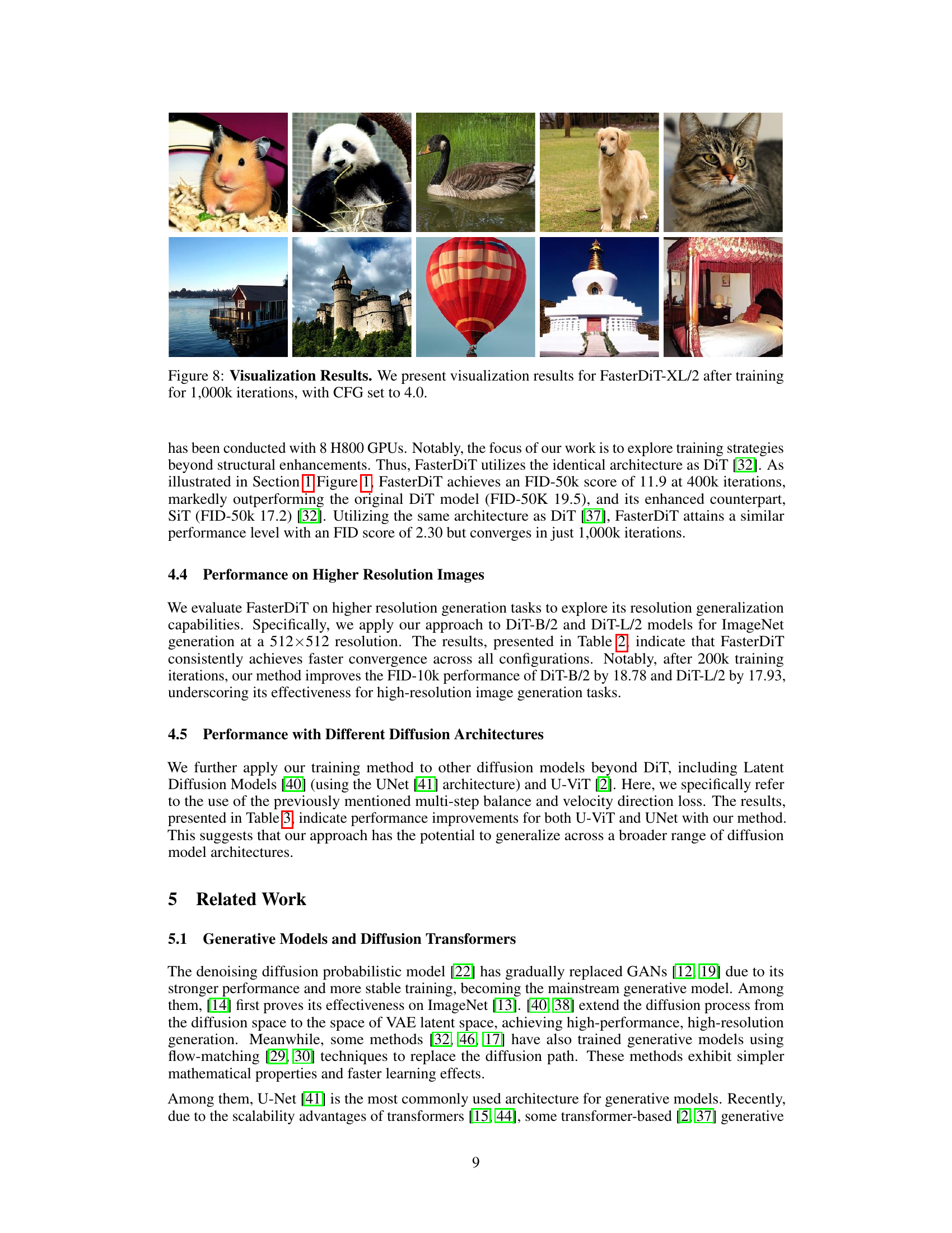
🔼 This figure shows several images generated by the FasterDiT-XL/2 model after training for 1,000,000 iterations with a CFG (classifier-free guidance) scale of 4.0. The images demonstrate the model’s ability to generate high-quality and diverse images across different categories, showcasing its performance after training.
read the caption
Figure 8: Visualization Results. We present visualization results for FasterDiT-XL/2 after training for 1,000k iterations, with CFG set to 4.0.

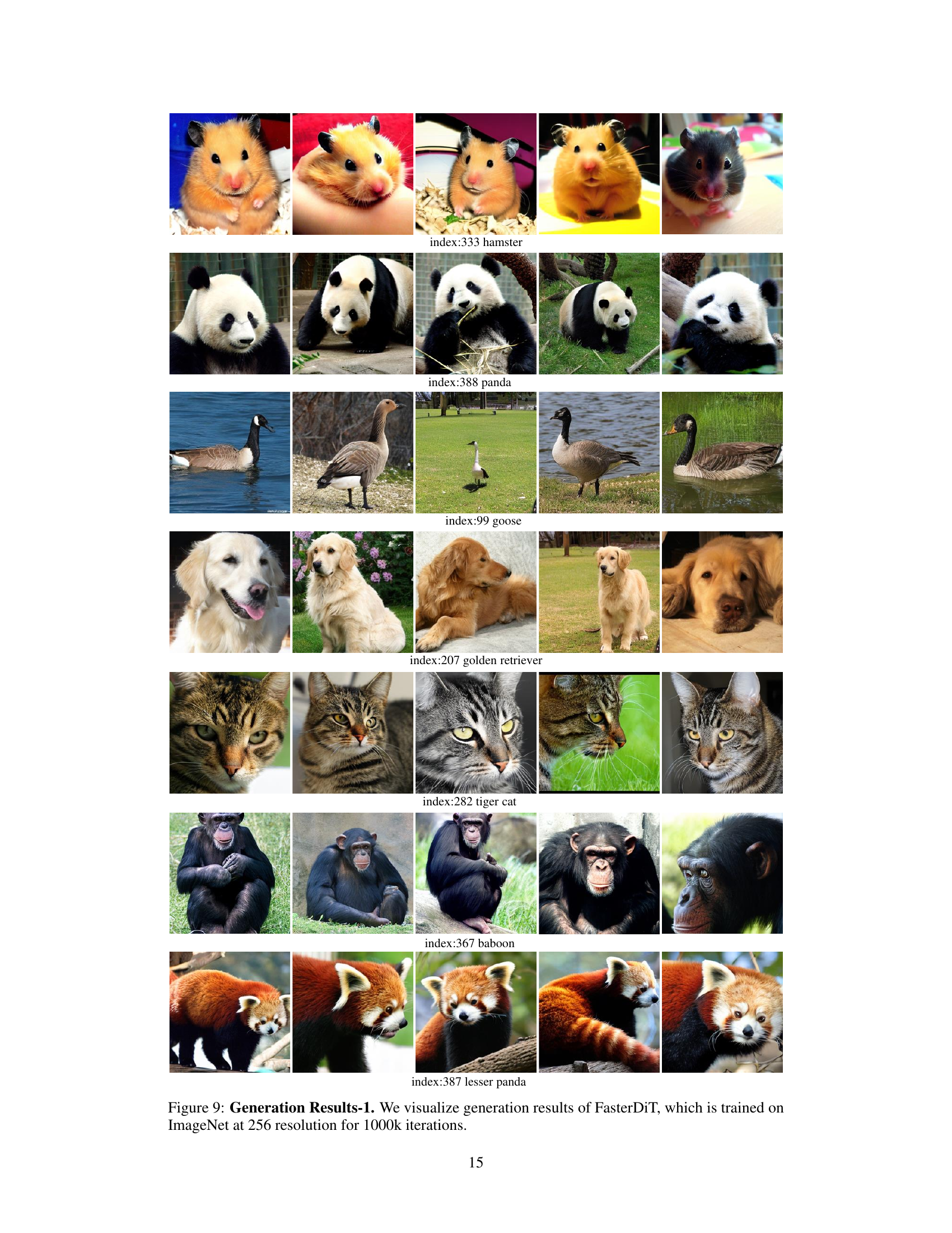
🔼 This figure shows several image generation results from the FasterDiT model. The model was trained on the ImageNet dataset at 256x256 resolution for 1,000,000 iterations. The images are categorized by their ImageNet index number and are representative samples showcasing the model’s performance in generating various animal images.
read the caption
Figure 9: Generation Results-1. We visualize generation results of FasterDiT, which is trained on ImageNet at 256 resolution for 1000k iterations.

🔼 This figure shows several example images generated by the FasterDiT model after training on the ImageNet dataset at a resolution of 256 for 1,000,000 iterations. The images are grouped by class and show the model’s ability to generate high-quality, diverse samples. It demonstrates the visual results obtained with FasterDiT after 1M iterations of training on ImageNet.
read the caption
Figure 10: Generation Results-2. We visualize generation results of FasterDiT, which is trained on ImageNet at 256 resolution for 1000k iterations.
More on tables

🔼 This table displays ablation studies conducted to analyze the impact of two key modifications to the training pipeline on the FID-50k score. The first modification is ‘multi-step balance’, and the second is ‘velocity direction loss’. The table shows the FID-50k scores achieved at 150k, 200k, and 400k training steps with different combinations of these modifications, demonstrating their effects on training efficiency.
read the caption
Table 7: Training Details. Our training pipeline involves only minimal modifications to the code.
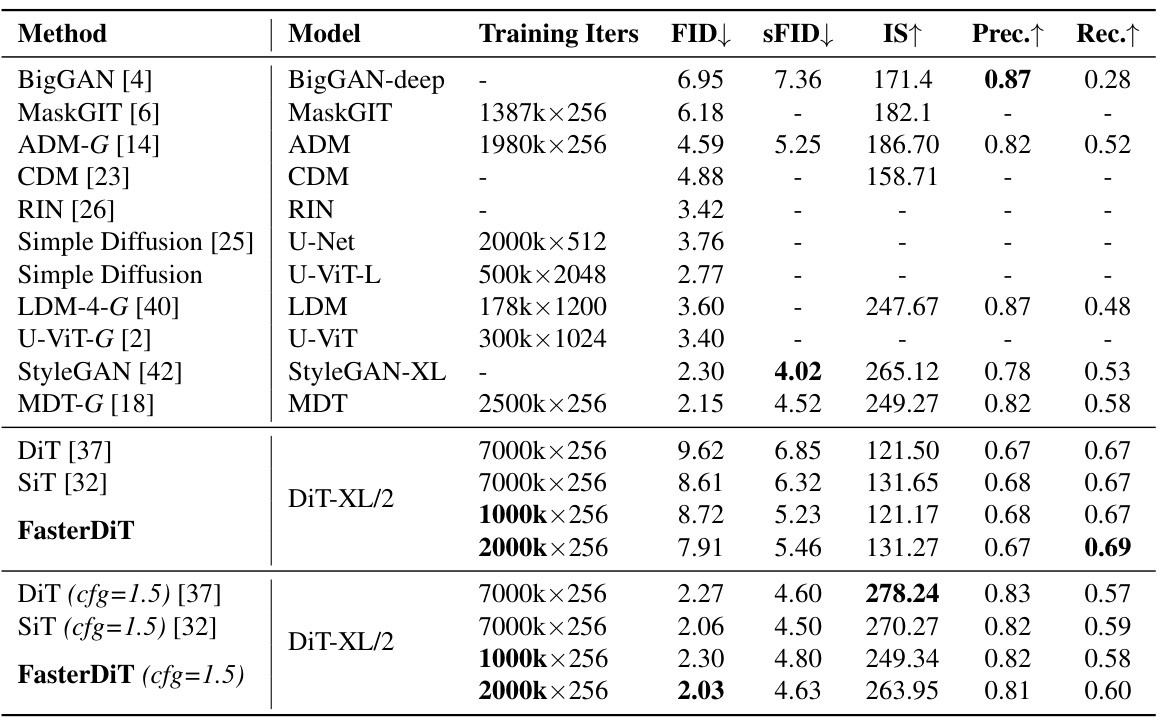
🔼 This table compares the performance of FasterDiT with other state-of-the-art image generation models on the ImageNet dataset at a resolution of 256x256. The key metrics compared are FID (Frechet Inception Distance), which measures the similarity between generated images and real images, and Inception Score (IS), which measures the quality and diversity of the generated images. FasterDiT shows a comparable FID score to other top-performing models but achieves this in significantly fewer training iterations, highlighting its improved training efficiency. The table also includes other metrics such as sFID, Precision, and Recall.
read the caption
Table 1: Performance of FasterDiT on ImageNet 256×256. Employing the identical architecture as DiT [37], FasterDiT achieves comparable performance with an FID of 2.30, yet requires only 1,000k iterations to converge.

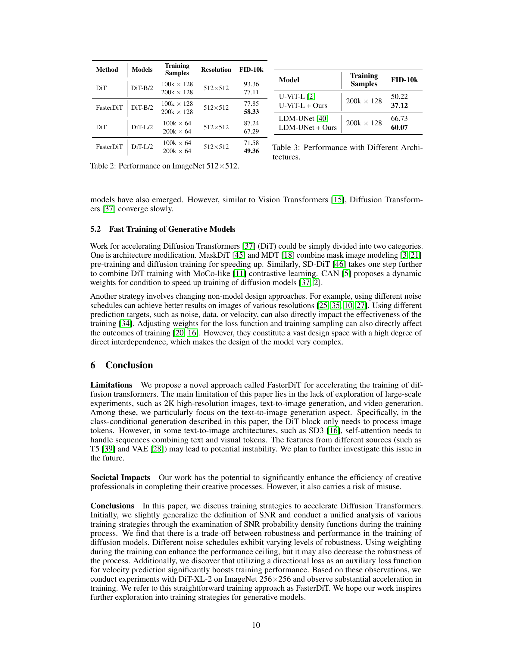
🔼 This table shows the performance of FasterDiT when applied to different diffusion model architectures beyond DiT, including Latent Diffusion Models (LDM) using the UNet architecture and U-ViT. The results demonstrate improvements in FID-10k scores for both U-ViT and UNet when using FasterDiT’s training methodology, suggesting that the approach can generalize across a broader range of architectures.
read the caption
Table 3: Performance with Different Architectures
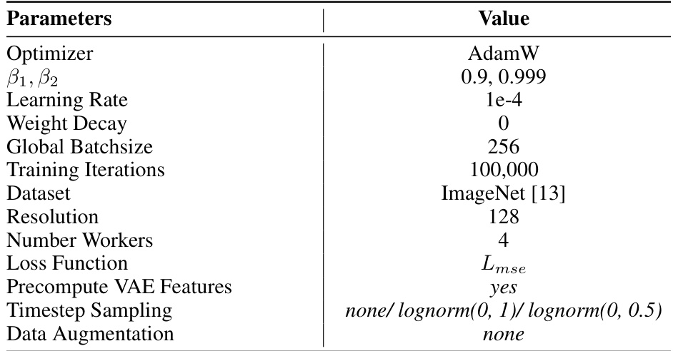
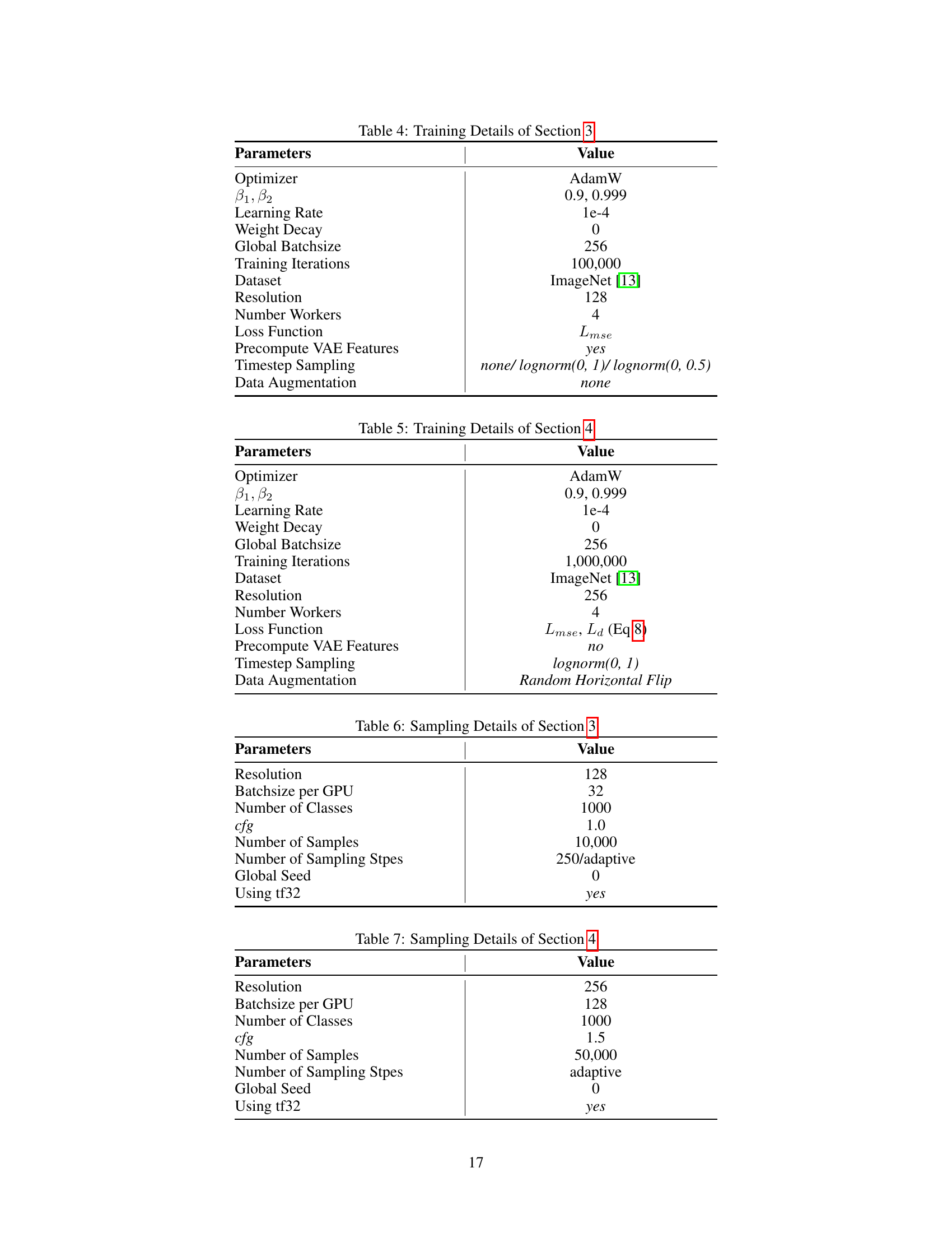
🔼 This table details the hyperparameters used for training the model in Section 3 of the paper. It includes specifications for the optimizer, learning rate, weight decay, batch size, number of training iterations, dataset used, image resolution, number of workers utilized for parallel processing, loss function, pre-computation of VAE features, timestep sampling strategy and data augmentation techniques. This information is crucial for understanding the experimental setup of the experiments presented in that section.
read the caption
Table 4: Training Details of Section 3

🔼 This table shows the hyperparameters used in the training process of the FasterDiT model in Section 4 of the paper. It includes details such as the optimizer, learning rate, weight decay, batch size, number of training iterations, dataset used, image resolution, number of workers, loss function, whether VAE features were precomputed, the timestep sampling strategy, and data augmentation techniques.
read the caption
Table 5: Training Details of Section 4

🔼 This table presents the hyperparameters used for sampling in Section 3 of the paper. It details the resolution, batch size per GPU, number of classes, CFG scale, number of samples, number of sampling steps, global seed, and whether tf32 was used.
read the caption
Table 6: Sampling Details of Section 3
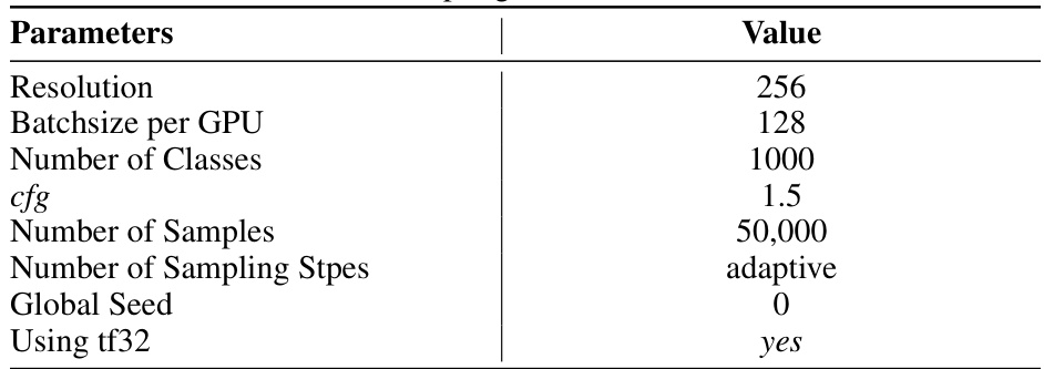
🔼 This table lists the hyperparameters used for sampling in Section 4 of the paper. It details settings for resolution, batch size per GPU, number of classes, CFG (classifier-free guidance) scale, the number of samples used for evaluation, the adaptive sampling step scheme, the global random seed, and the use of tf32 precision.
read the caption
Table 7: Sampling Details of Section 4
Full paper#

