↗ OpenReview ↗ NeurIPS Homepage ↗ Chat
TL;DR#
Current deep learning approaches for time series forecasting show inconsistent scaling behaviors. While larger datasets generally improve performance, larger models and longer input horizons don’t always lead to better results, challenging the widely observed scaling laws in other deep learning fields. This inconsistency is a significant hurdle for researchers seeking to develop robust and efficient forecasting models.
This paper introduces a new theoretical framework explaining these anomalies by incorporating the impact of the ’look-back horizon’ – the length of past data considered. Through empirical evaluation across diverse datasets and models, the researchers validated their theory, revealing an optimal look-back horizon that increases with dataset size. Their findings provide valuable insights for building more effective models, particularly for datasets of limited size, while also advocating for the development of larger foundational datasets and models.
Key Takeaways#
Why does it matter?#
This paper is crucial because it challenges existing assumptions about scaling laws in time series forecasting and provides a more nuanced understanding. By identifying the optimal horizon and its relation to dataset size and model complexity, it guides researchers in designing better models for both limited and large datasets, stimulating further research into efficient time series modeling.
Visual Insights#
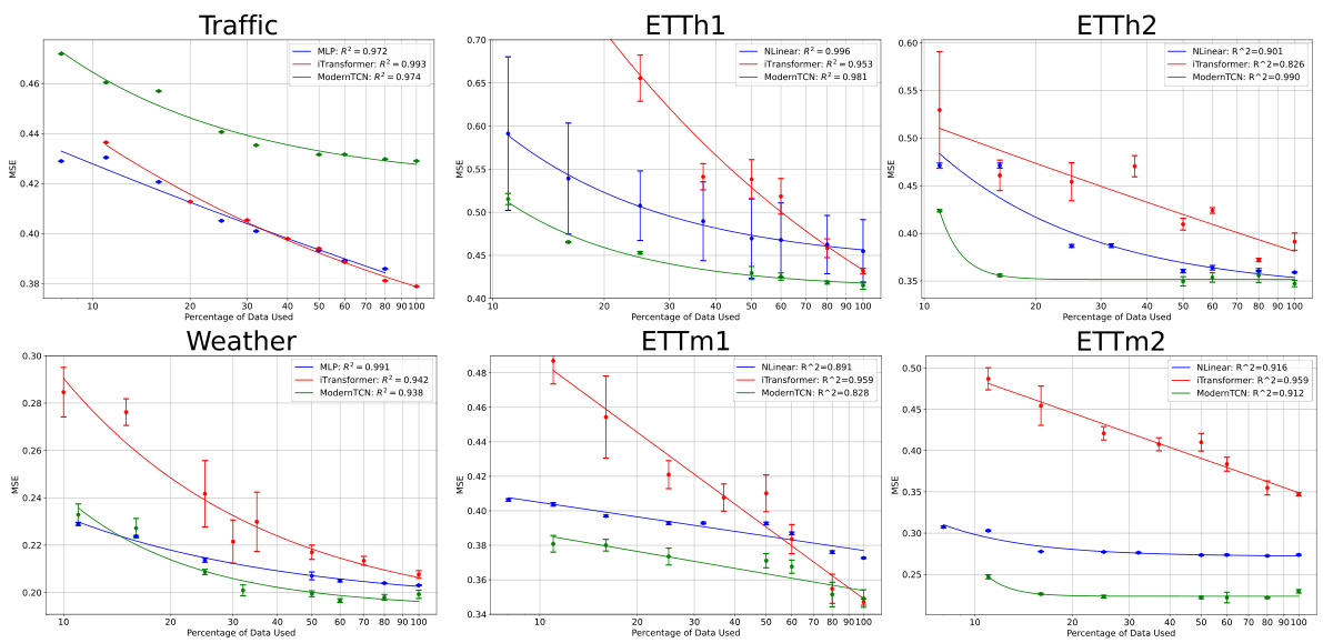
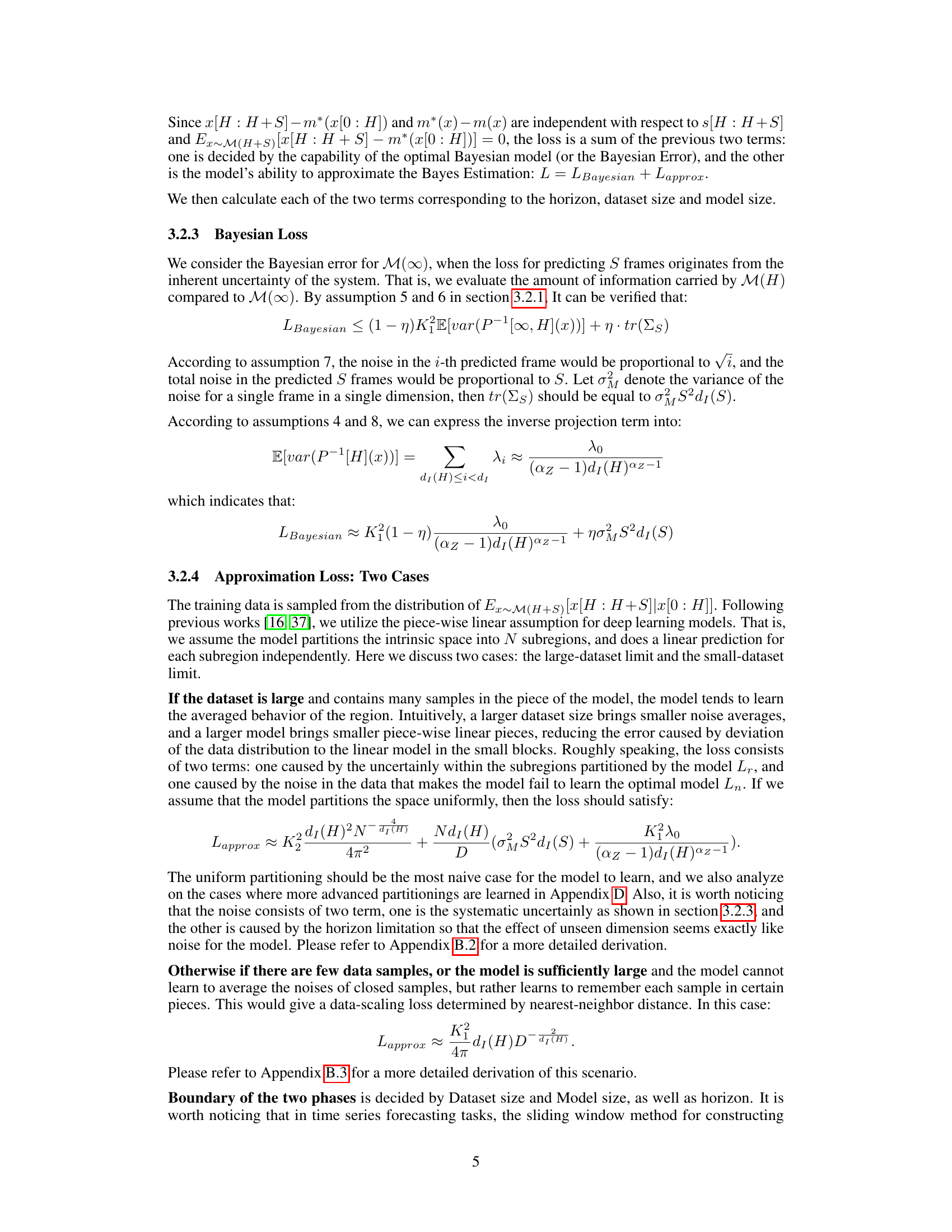
This figure shows the results of experiments on data scaling. The x-axis represents the percentage of data used for training, and the y-axis represents the loss. The figure shows that the proposed formula, loss(D) = A + B/D^α, provides a good fit for the data, where D represents the dataset size and α is a scaling exponent. Different lines on the graph represent different time series forecasting models and datasets. The caption indicates that additional comparisons with other formulas can be found in Appendix I of the paper.

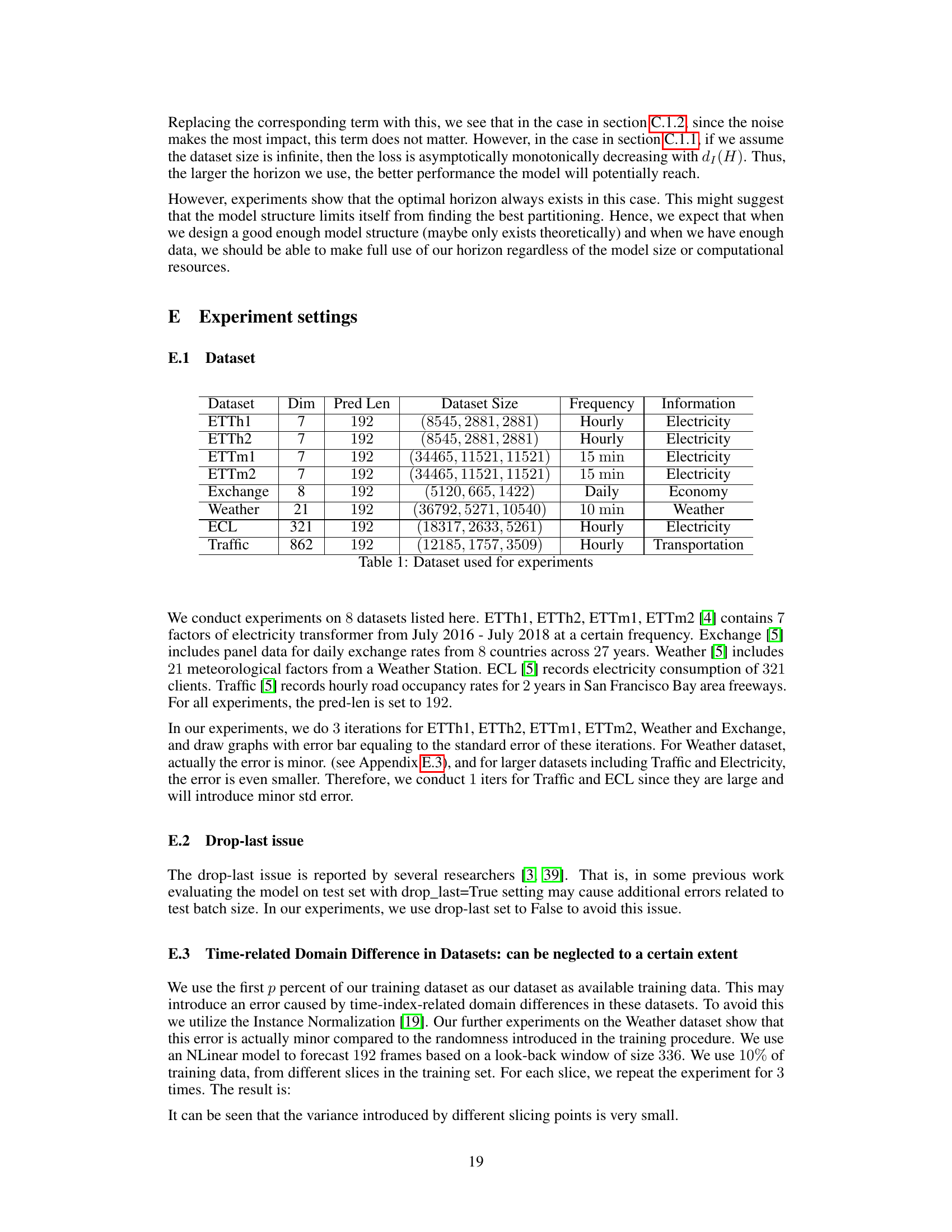
This table lists the eight datasets used in the paper’s experiments. For each dataset, it provides the number of dimensions (Dim), prediction length (Pred Len), dataset size (broken down into training, validation, and test sets), frequency of data points (Hourly, Daily, 10 min, 15 min), and the type of information the data represents (Electricity, Economy, Weather, Transportation). These datasets are used to evaluate the scaling laws and models for time series forecasting.
In-depth insights#
Time Series Scaling#
The concept of “Time Series Scaling” in the context of deep learning for time series forecasting investigates how model performance changes with respect to various factors such as dataset size, model complexity, and data granularity (lookback horizon). The authors challenge the common assumption that larger models and longer horizons always lead to better results. Their proposed theory integrates these factors to explain seemingly abnormal scaling behaviors, suggesting that an optimal horizon exists and is influenced by dataset size. Empirical results across various models and datasets support the existence of scaling laws for dataset size and model complexity, and validate their theoretical framework regarding the impact of the lookback horizon. The study highlights the importance of considering these interwoven factors for improved forecasting model design, particularly when dealing with limited data or computational resources. The work suggests that using a longer lookback horizon than optimal can negatively impact performance, emphasizing the need for more careful model design and parameter tuning tailored to specific datasets and computational constraints.
Intrinsic Space Theory#
The proposed Intrinsic Space Theory offers a novel perspective on scaling laws in time series forecasting, moving beyond simple dataset and model size considerations. It cleverly introduces the concept of an intrinsic space, representing the fundamental information embedded within time series data slices of a specific length. This framework elegantly accounts for the impact of the look-back horizon, a crucial element previously neglected in scaling law analyses. By establishing a relationship between the intrinsic dimension of this space and the look-back horizon, the theory explains seemingly contradictory observations, such as the non-monotonic relationship between input length and forecasting performance. The theory leverages the concept of intrinsic dimension to quantify information content, suggesting that forecasting performance hinges on the ability of the model to capture this information. Importantly, the theory differentiates between regimes of data abundance and scarcity, proposing that optimal horizon shifts based on dataset size. This is a significant contribution as it tackles the inherent challenges of limited data in many practical time series applications. Ultimately, the Intrinsic Space Theory provides a more nuanced and comprehensive understanding of scaling effects in time series forecasting, paving the way for improved model design and data handling strategies.
Horizon’s Impact#
The concept of ‘Horizon’s Impact’ in time series forecasting is crucial. It examines how the length of the input sequence (look-back horizon) affects forecasting accuracy. Longer horizons provide more historical data, potentially improving model learning and predictive power. However, excessively long horizons can lead to increased computational costs, noise in older data, and overfitting. The paper investigates the optimal horizon, demonstrating that this optimal length isn’t fixed but depends on factors such as dataset size and model complexity. A smaller dataset may be overwhelmed by excessive historical data, while a complex model might be more susceptible to overfitting. The study thus advocates for an adaptive approach, adjusting the horizon dynamically depending on the characteristics of the dataset and model. This nuanced perspective reveals the significant role of horizon in practical applications, where the balance between data richness and computational constraints must be carefully considered for optimal forecasting performance. This adaptive method helps to obtain the best prediction accuracy while being computationally feasible.
Empirical Validation#
The empirical validation section of a research paper should rigorously test the proposed theory or model. This involves carefully selecting diverse and representative datasets to avoid bias and ensure generalizability. The section should clearly outline the experimental setup, including metrics used, baseline models for comparison, and the methodology for evaluating results. Statistical significance should be explicitly addressed to ensure that observed results are not due to chance. The authors should meticulously discuss any limitations of the experiments, potential biases, and their impact on the interpretations of the results. A robust empirical validation bolsters the credibility of the research by providing concrete evidence to support the claims made, which enhances the overall impact and significance of the study. Visualizations like graphs and tables are essential to effectively communicate the results and facilitate understanding for the readers. Transparency in data handling, clear description of methodology and results analysis are key factors for a convincing empirical validation.
Future Directions#
Future research directions stemming from this scaling law analysis for time series forecasting could fruitfully explore several avenues. Extending the theoretical framework to encompass more complex scenarios, such as multivariate time series with non-linear relationships or those exhibiting seasonality and trends, is crucial. Empirical validation should be pursued using substantially larger, more diverse datasets to test the generalizability of the proposed scaling law. Investigating the interplay between different model architectures and their respective optimal look-back horizons merits further attention. Advanced model architectures designed specifically to handle the challenges posed by limited data or high-dimensional intrinsic spaces should also be explored. The optimal horizon’s sensitivity to data characteristics like noise levels, outliers, or feature dimensionality warrants careful study. Finally, developing practical guidelines that leverage this scaling law for model selection and hyperparameter tuning in real-world applications would provide significant practical value.
More visual insights#
More on figures

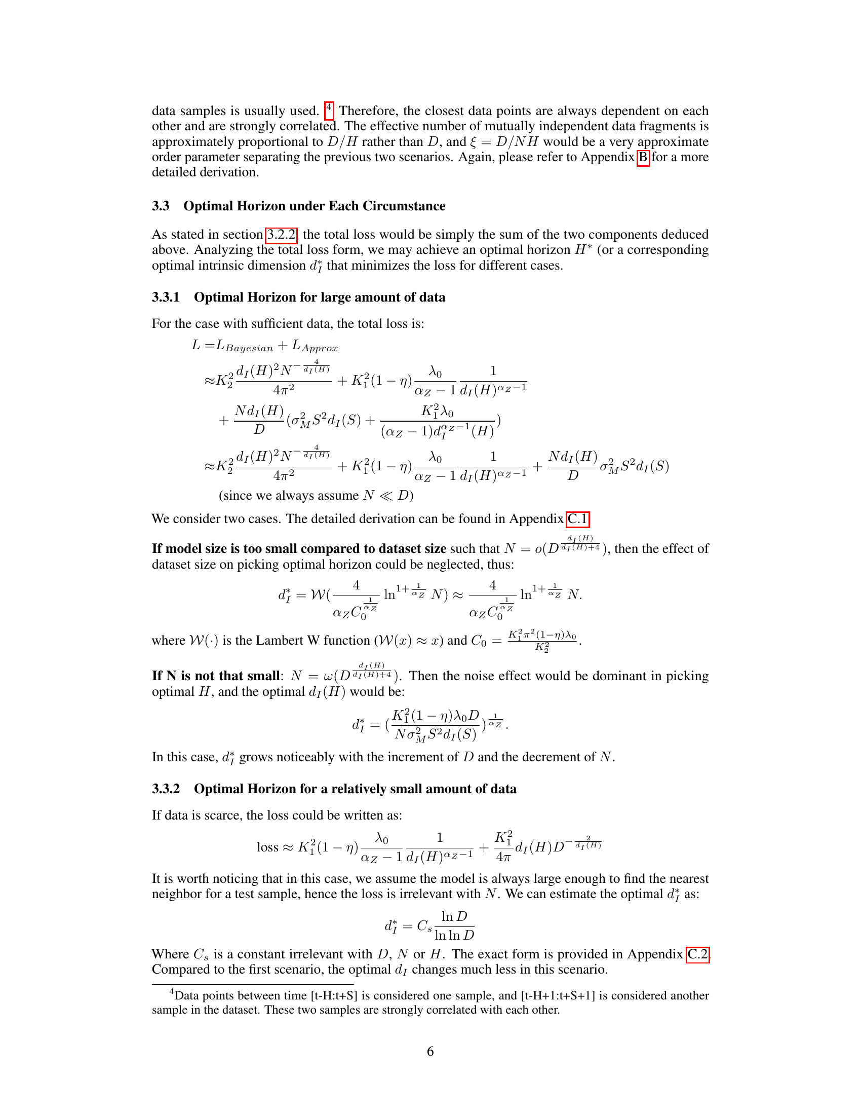
This figure shows the results of experiments on the impact of model width on the loss function for time series forecasting. It confirms that increasing model width generally reduces loss, following a power law relationship (loss(W) = A + B/W^α) when the model is not too large. However, when data is scarce (as with the ModernTCN model on the ETTm1 dataset), very large models can lead to overfitting and increased loss, indicating an optimal model width exists.
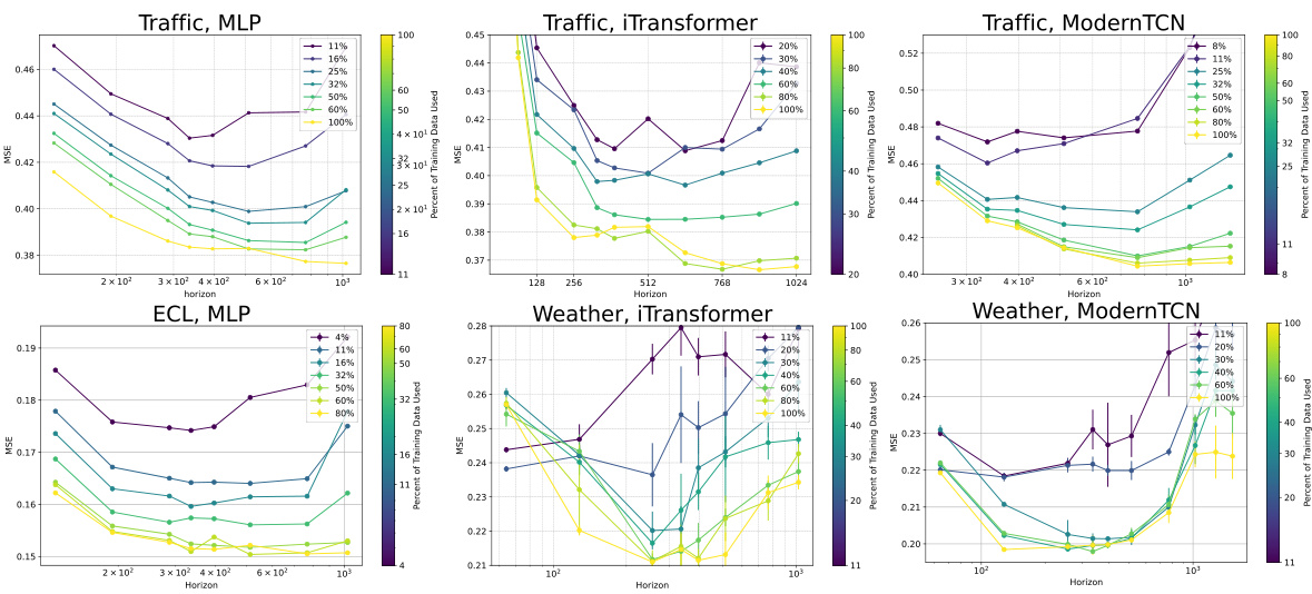
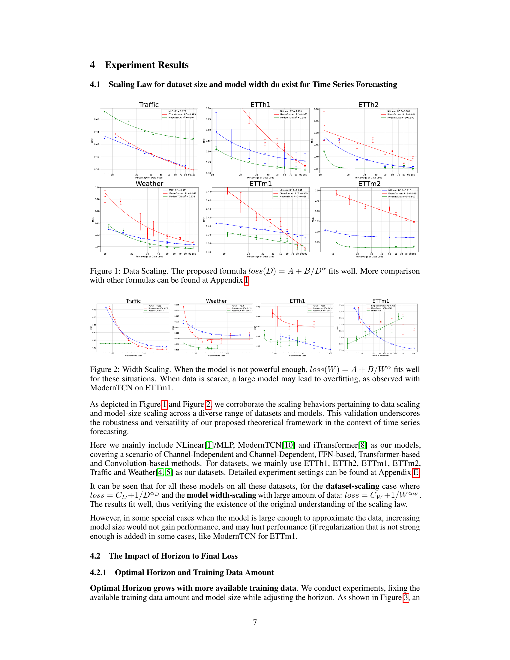
This figure displays the relationship between loss and horizon for various datasets and models, each with a specific amount of training data. It demonstrates how the optimal horizon (the point at which loss is minimized) changes depending on the amount of available training data. The figure helps visualize the impact of the look-back horizon on model performance in time series forecasting. Different lines represent different amounts of training data used for each model.

This figure shows the results of experiments on data scaling in time series forecasting. It validates the scaling law theory proposed in the paper by demonstrating a relationship between dataset size (D) and loss. The formula loss(D) = A + B/Dº, where A and B are constants and α is the scaling exponent, is shown to provide a good fit for the data. Appendix I contains additional comparisons of this formula with other possible formulas.

This figure shows the results of experiments on data scaling for time series forecasting. The x-axis represents the percentage of data used, and the y-axis represents the loss. Multiple lines represent different models tested on various datasets. The caption indicates that the proposed formula, loss(D) = A + B/D^α, provides a good fit to the data, and additional comparisons using different formulas are available in Appendix I. The figure demonstrates that performance improves with increasing data size, which is a key finding of the scaling law.

This figure displays the results of experiments on data scaling in time series forecasting. It shows the relationship between the size of the dataset (D) and the loss for different models on various datasets (Traffic, Weather, ETTh1, ETTh2, ETTm1, ETTm2). The results demonstrate that the proposed formula loss(D) = A + B/D^α provides a good fit for the observed data. Appendix I contains a more detailed comparison with other formulas.
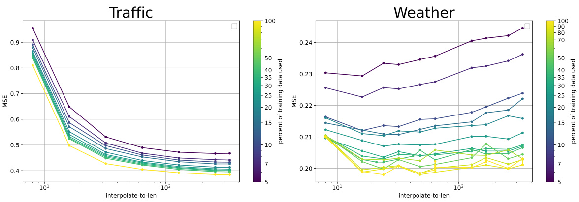
This figure shows the impact of downsampling on the MSE loss for Traffic and Weather datasets. The x-axis represents the length after downsampling, while the y-axis represents the MSE loss. Different colored lines represent different amounts of training data used. The figure visually demonstrates how downsampling affects model performance, which is explained in Section F of the paper.
This figure displays the results of data scaling experiments. It shows that the relationship between dataset size (D) and loss follows a power law, as indicated by the proposed formula loss(D) = A + B/D^α. The figure includes multiple subplots, each showing the results for a different time series dataset (Traffic, Weather, ETTh1, ETTh2, ETTm1, ETTm2). Each subplot shows the loss on the y-axis and the percentage of data used on the x-axis. The strong fit of the proposed power law formula suggests a scaling law behavior for dataset size in time series forecasting exists.
This figure shows the results of experiments on data scaling. The x-axis represents the percentage of data used, while the y-axis represents the loss. Different lines represent different models (MLP, iTransformer, ModernTCN) applied to different datasets (Traffic, Weather, ETTh1, ETTh2, ETTm1, ETTm2). The figure demonstrates that the proposed formula loss(D) = A + B/D^α provides a good fit to the experimental data, validating the scaling law for dataset size in time series forecasting. Appendix I contains further comparisons with other formulas.

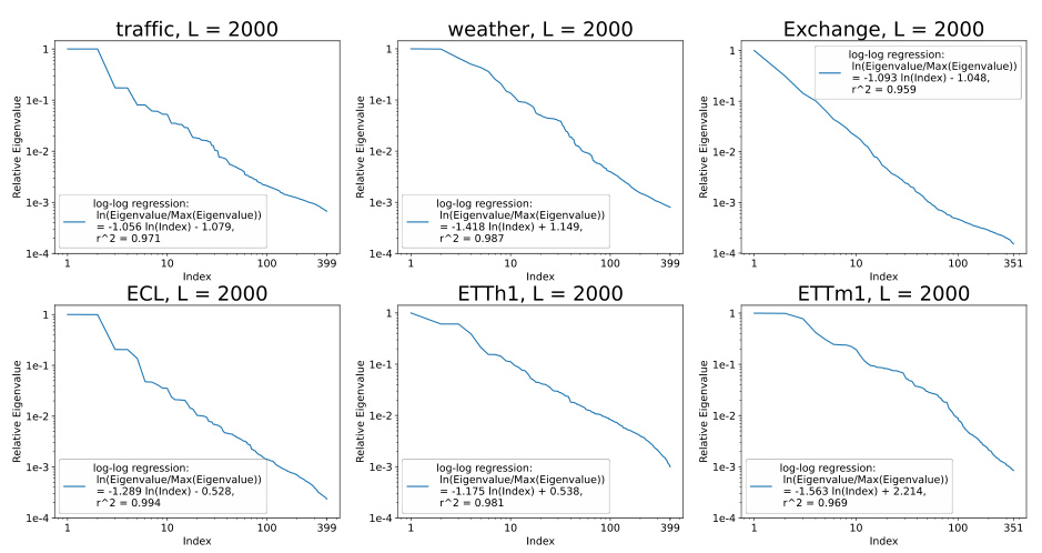
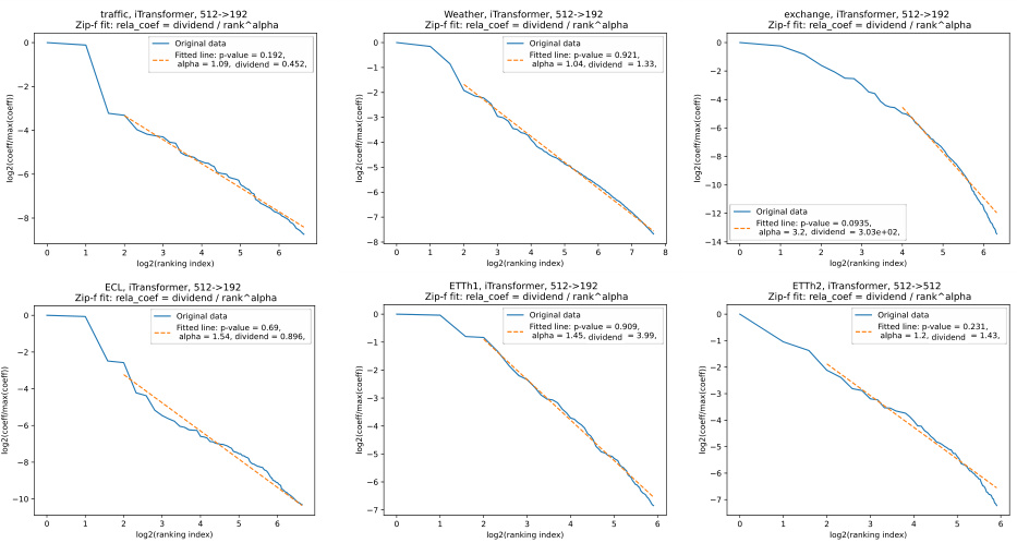
This figure displays the results of Principal Component Analysis (PCA) performed on features extracted from a Multilayer Perceptron (MLP) model trained on a mixed dataset. The dataset combines various time series datasets, including Traffic, Weather, Exchange, ETTh1, ETTh2, ETTm1, ETTm2, and ECL. The analysis reveals that the resulting feature distribution closely follows a Zipf’s law, particularly for features with higher rankings. This finding is consistent with the paper’s theoretical framework, which postulates that data distribution within the intrinsic space follows a Zipf’s law.
More on tables

This table shows the Mean Squared Error (MSE) for the Weather dataset. Multiple experiments (Exp1, Exp2, Exp3) were run, each starting at a different percentage point of the training data (20%, 40%, 60%, 80%). The average MSE and standard deviation are calculated for each starting point, demonstrating the impact of available training data on model performance.

This table presents the AIC and BIC values for four different formulas that were used to fit the loss curves for the ModernTCN model. The formulas tested were: f(x) = A + B/x^α, g1(x) = A/x^α, g2(x) = A + B log(x), and g3(x) = A + Bx + Cx^2. The AIC and BIC values are provided for each formula and for four different datasets: Traffic, Weather, ETTh1, and ETTh2.

This table presents the AIC and BIC values resulting from fitting four different regression formulas to the loss function of the iTransformer model. The formulas are applied to four different datasets: Traffic, Weather, ETTh1, and ETTh2. The AIC and BIC values provide a measure of the goodness of fit for each formula on each dataset, helping to assess which formula best captures the relationship between the model’s parameters and its performance.

This table presents the AIC and BIC values resulting from fitting four different regression formulas (f, g1, g2, g3) to time series forecasting data from four datasets (Traffic, Weather, ETTh1, ETTh2). The formulas represent different modeling approaches, and the AIC and BIC values provide a measure of the relative goodness of fit for each formula on each dataset. Lower AIC and BIC values indicate better model fit.
Full paper#
