↗ OpenReview ↗ NeurIPS Homepage ↗ Chat
TL;DR#
Generative AI for tabular data faces challenges with model selection and training. Existing models struggle with efficiency and theoretical guarantees. Neural nets dominate unstructured data but underperform on tabular data in many cases.
This research introduces Generative Forests (GFs), a novel class of forest-based models, along with a simple, theoretically-sound training algorithm (GF.BOOST). GF.BOOST minimizes losses efficiently and the model structure facilitates fast density estimations. Experiments demonstrate that GFs produce substantially better results than state-of-the-art methods in data generation, imputation, and density estimation. The algorithm’s simplicity and theoretical guarantees are key strengths. Significant improvements are demonstrated across various tasks.
Key Takeaways#
Why does it matter?#
This paper is crucial for researchers in machine learning and data science due to its novel approach to generative AI for tabular data, a common yet challenging data type. The simple yet powerful algorithm, with strong theoretical guarantees, provides a significant improvement in data generation quality and offers practical solutions for crucial tasks like missing data imputation and density estimation. It opens new avenues for research into boosting models for generative AI and may greatly impact future developments in the field.
Visual Insights#

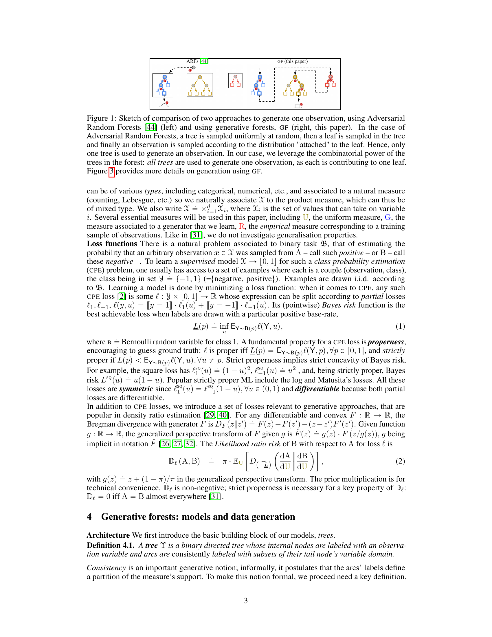
The figure compares two methods for generating data: Adversarial Random Forests (ARFs) and Generative Forests (GFs). ARFs use only one tree to generate each observation, while GFs utilize all trees in the forest, leveraging the combinatorial power for improved data generation.

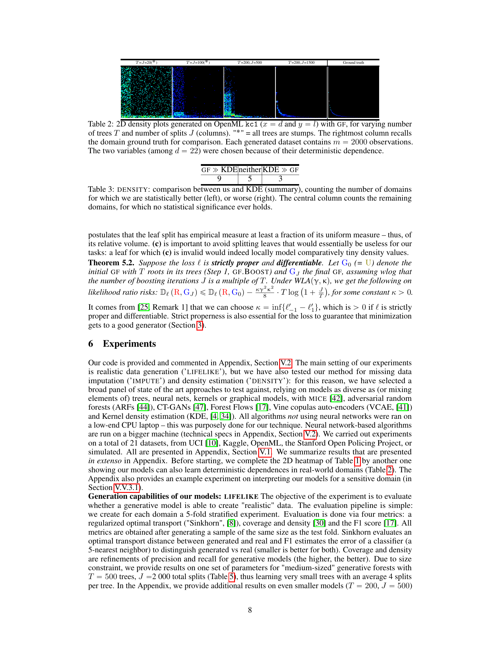
This table compares the density learned by three different generative forest models on the circgauss domain. The first model uses a single tree boosted for 50 iterations, the second model uses 50 boosted tree stumps, and the third model is the ground truth. The table shows that a set of tree stumps can learn a much more accurate density than a single tree, even if each tree in the set of stumps is very simple. This is because the set of stumps can partition the domain into many more parts than a single tree.
In-depth insights#
Tabular Data Gen#
The heading ‘Tabular Data Gen’ likely refers to the generation of synthetic tabular data, a significant challenge in machine learning. Generating realistic tabular data is crucial for various applications such as data augmentation, privacy-preserving data sharing, and testing new algorithms. The core difficulty lies in capturing the complex relationships between variables, including dependencies and conditional probabilities, which often exhibit non-linear patterns. Existing methods have limitations in accurately modeling these intricate relationships and often struggle to generate high-quality, diverse datasets. The research likely explores novel approaches to tabular data generation, potentially leveraging techniques such as deep generative models, probabilistic graphical models, or advanced tree-based methods. A key focus might be on developing efficient training algorithms and evaluating the quality of the generated data against standard metrics. The analysis likely assesses the effectiveness of the proposed method in comparison to existing state-of-the-art techniques, showcasing improvements in the quality and diversity of synthetic tabular data generated. Strong convergence guarantees and scalability are likely important aspects considered in the research.
GF Architecture#
Generative Forests (GFs) are a novel class of forest-based models designed for generative AI tasks on tabular data. The GF architecture is tree-based, building upon the popular induction scheme for decision trees, but with crucial modifications to accommodate the generative setting. Instead of a single tree as in previous generative tree models, GFs employ an ensemble of trees, leveraging the combinatorial power of multiple trees to achieve richer data generation capabilities. Each tree in the ensemble contributes independently to the overall generative process, leading to substantial improvements compared to the state-of-the-art. A key component of the GF architecture is the concept of consistency, which ensures that the partitioning of the feature space by the ensemble is well-defined. This, along with the specific loss function optimized by the training algorithm, contributes to the model’s efficacy in various generative AI tasks, such as density estimation and missing data imputation. The simplicity of implementation combined with strong theoretical guarantees makes the GF architecture a promising approach for addressing the challenges of generative AI in the context of tabular data.
Supervised Boosting#
The concept of “Supervised Boosting” in the context of generative models for tabular data presents a novel approach to training. Instead of relying on the adversarial framework common in Generative Adversarial Networks (GANs), this method leverages a supervised learning setting. This is achieved by framing the problem as a binary classification task: distinguishing between real data and data generated by the model. A key advantage is the elimination of the inherent slack between generator and discriminator losses often found in GANs. The algorithm minimizes a loss function that is closely related to the likelihood ratio risk, providing strong convergence guarantees and parallels to the original boosting model’s weak/strong learning paradigm. The simplicity of this method allows implementation with minimal changes to standard decision tree induction schemes, making it highly practical and efficient. The theoretical guarantees further enhance its robustness. While the exact mathematical details would depend on the specific implementation, the core idea of using supervised boosting offers significant advantages in stability and efficiency compared to adversarial training within the context of tabular data generation.
Missing Data Imputation#
The research paper explores missing data imputation within the context of generative forests. Generative forests, a novel class of models, are shown to be effective at imputing missing values, potentially outperforming existing methods like MICE (Multiple Imputation by Chained Equations). The paper highlights the simplicity and efficiency of the proposed imputation algorithm, which leverages the inherent structure of the generative forest models. Importantly, the method’s efficacy is demonstrated across various datasets with different characteristics, underscoring its robustness and generalizability. The paper also contrasts its approach with other state-of-the-art techniques and showcases how the strong theoretical guarantees of the generative forest training algorithm translate to better performance in missing data imputation tasks. Further investigation reveals that the models, despite their simplicity, can achieve comparable performance to more complex methods, especially for smaller datasets. Practical advantages of the approach include its speed and ease of implementation, making it suitable for large-scale applications.
Future Work#
The research paper’s “Future Work” section could explore several promising avenues. Improving the theoretical framework is crucial, potentially relaxing assumptions like boundedness or Lipschitz continuity to better handle real-world data. Developing more efficient training algorithms is another key area; investigating alternative optimization strategies and pruning techniques could dramatically reduce computational costs. The work could also be extended to explore the potential of generative forests for diverse tasks such as anomaly detection, causal inference, and reinforcement learning. Further research should focus on developing methods to automatically determine optimal model size, balancing accuracy and efficiency. Finally, exploring hybrid models combining generative forests with other architectures (e.g., neural networks) could lead to significant improvements in performance. Addressing these aspects would significantly advance this promising field.
More visual insights#
More on figures

This figure compares two methods for generating data: Adversarial Random Forests (ARFs) and Generative Forests (GFs). ARFs randomly select a tree from a forest, sample a leaf from that tree, and then generate an observation based on the leaf’s distribution. GFs use all trees in the forest simultaneously to generate a single observation, leveraging the combinatorial power of the trees to create a more diverse and potentially higher-quality data set.

The figure compares two methods for generating data: Adversarial Random Forests (ARFs) and Generative Forests (GFs). ARFs randomly select a tree, then a leaf within that tree, and finally sample an observation from the leaf’s distribution. This means only one tree contributes to each generated observation. GFs utilize all trees in the forest; each tree contributes a leaf, and the generated observation comes from the intersection of all these leaves. This leverages the combined power of all trees for each observation.

This figure compares two methods for generating data: Adversarial Random Forests (ARFs) and Generative Forests (GFs). ARFs randomly select a tree, then a leaf from that tree, and finally sample an observation from that leaf’s distribution. In contrast, GFs utilize all trees in the forest to generate a single observation, improving data diversity.

The figure compares two methods for generating data: Adversarial Random Forests (ARFs) and Generative Forests (GFs). ARFs randomly select a tree, then a leaf within that tree, and sample from the leaf’s distribution. GFs use all trees in the forest, combining the information from the leaves of all trees to generate a single observation.

This figure compares two methods for generating data: Adversarial Random Forests (ARFs) and Generative Forests (GFs). ARFs randomly select a tree from a forest, then sample a leaf from that tree, and finally generate an observation based on the leaf’s distribution. In contrast, GFs utilize all trees in the forest to generate a single observation. Each tree contributes information, resulting in a more comprehensive and potentially more accurate data generation process.

This figure compares two methods for generating data: Adversarial Random Forests (ARFs) and Generative Forests (GFs). ARFs randomly select a tree, sample a leaf from that tree, and generate data based on that leaf’s distribution. In contrast, GFs utilize all trees in the forest to generate a single observation. Each tree contributes a leaf to the process, and the final observation is generated based on the combination of all leaves. This highlights the combinatorial advantage of GFs over ARFs.
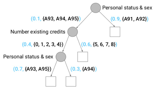
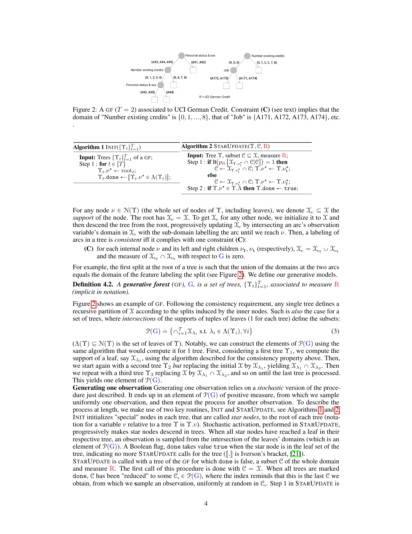
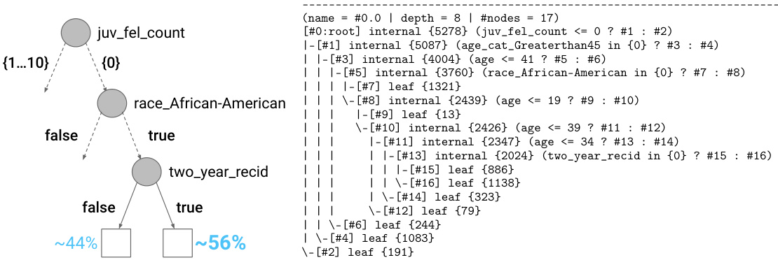
This figure shows a generative forest (GF) with two trees (T=2) applied to the UCI German Credit dataset. The figure highlights how the trees recursively partition the feature space based on the values of the features. Each node represents a decision point, splitting the data based on a feature’s value. The numbers in parentheses represent probabilities of taking a certain path down the tree, and the sets represent the allowed values of the features in that part of the tree. This example visually illustrates the consistent partitioning of the feature space that the GF’s consistency constraint (C) enforces.
This figure compares two methods for generating data: Adversarial Random Forests (ARFs) and Generative Forests (GFs). ARFs randomly select a tree, sample a leaf from that tree, and then sample an observation from the distribution associated with the leaf. GFs use all trees in the forest to generate a single observation, leveraging the combinatorial power of the ensemble.

This figure compares two methods for generating data: Adversarial Random Forests (ARFs) and Generative Forests (GFs). ARFs randomly select a tree, then a leaf from that tree, and finally sample data from the leaf’s distribution. In contrast, GFs use all trees in the forest to generate a single data point, combining information from leaves across all trees for greater efficiency and accuracy.

This figure compares two methods for generating data: Adversarial Random Forests (ARFs) and Generative Forests (GFs). ARFs randomly select a tree, sample a leaf from that tree, and generate an observation based on that leaf’s distribution. GFs, in contrast, use all trees in the forest to generate a single observation, leveraging the combinatorial power of the trees.

This figure compares two methods for generating data: Adversarial Random Forests (ARFs) and Generative Forests (GFs). ARFs select a single tree at random and sample an observation from a leaf of that tree. In contrast, GFs use all trees in the forest to generate each observation. This combinatorial approach allows GFs to capture more complex data distributions.
This figure compares two methods for generating data: Adversarial Random Forests (ARFs) and Generative Forests (GFs). ARFs randomly select a tree, then a leaf within that tree, and finally sample an observation from the distribution associated with that leaf. In contrast, GFs utilize all trees in the forest, with each contributing to the generation of a single observation, leveraging the combinatorial power of the entire forest.

This figure compares two methods for generating data: Adversarial Random Forests (ARFs) and Generative Forests (GFs). ARFs randomly select a tree, then a leaf from that tree, and finally sample an observation from the leaf’s distribution. In contrast, GFs utilize all trees to generate a single observation by considering the combinatorial possibilities across all leaves.
This figure compares two methods for generating data: Adversarial Random Forests (ARFs) and Generative Forests (GFs). ARFs randomly select a tree from a forest, then a leaf from that tree, and finally sample an observation from the leaf’s distribution. GFs utilize all trees in the forest to generate a single observation, combining information from the leaves of each tree.
This figure compares two methods for generating data: Adversarial Random Forests (ARFs) and Generative Forests (GFs). ARFs randomly select a tree from the forest, then sample a leaf from that tree, and finally generate data based on the leaf’s distribution. GFs, on the other hand, utilize all trees in the forest simultaneously to generate a single data point. Each tree contributes a leaf, and the final data point is generated based on the intersection of all these leaves’ domains, leveraging the combinatorial power of the entire forest.

This figure compares two methods for generating data: Adversarial Random Forests (ARFs) and Generative Forests (GFs). ARFs randomly select a tree and sample from a leaf’s distribution. GFs use all trees to generate one observation by combining leaves’ information. GFs are shown to generate data more efficiently by leveraging the combinatorial power of multiple trees.

The figure compares two methods for generating data: Adversarial Random Forests (ARFs) and Generative Forests (GFs). ARFs randomly select a tree, then a leaf within that tree, and finally sample an observation from the leaf’s distribution. In contrast, GFs utilize all trees to generate a single observation by combining information from leaves across the entire forest.

This figure compares two methods for generating data: Adversarial Random Forests (ARFs) and Generative Forests (GFs). ARFs randomly select a tree, sample a leaf from that tree, and then generate data based on that leaf’s distribution. In contrast, GFs utilize all trees in the forest to generate a single observation, leveraging the combinatorial power of the entire ensemble. This difference highlights a key distinction between the two approaches.

This figure compares two methods for generating data: Adversarial Random Forests (ARFs) and Generative Forests (GFs). ARFs randomly select a tree, then a leaf from that tree, and finally sample an observation from the leaf’s distribution. GFs use all trees in the forest to generate a single observation, leveraging the combinatorial power of the multiple trees. The figure illustrates the different approaches visually.
The figure compares two methods for generating data: Adversarial Random Forests (ARFs) and Generative Forests (GFs). ARFs randomly select a tree from a forest, then a leaf from that tree, and finally sample an observation from the leaf’s distribution. In contrast, GFs use all trees in the forest to generate a single observation, leveraging the combinatorial power of the multiple trees.
This figure compares two methods for generating data: Adversarial Random Forests (ARFs) and Generative Forests (GFs). ARFs select a single tree at random and sample an observation from a leaf within that tree. In contrast, GFs use all trees in the forest; each tree contributes a leaf to the process of generating a single observation. This highlights the key difference between the two approaches: ARFs rely on individual trees to generate samples, whereas GFs leverage the collective power of the entire forest.

This figure compares two methods for generating data: Adversarial Random Forests (ARFs) and Generative Forests (GFs). ARFs randomly select a tree from the forest, then sample a leaf from that tree, and finally sample an observation from the distribution associated with the leaf. In contrast, GFs use all trees in the forest to generate a single observation. Each tree contributes a leaf, and the final observation is generated based on the combined information from all the leaves.

This figure compares two methods for generating data: Adversarial Random Forests (ARFs) and Generative Forests (GFs). ARFs randomly select a tree, sample a leaf from that tree, and then sample an observation from the leaf’s distribution. In contrast, GFs utilize all trees in the forest; each tree contributes to a leaf, and the final observation is generated from the intersection of all selected leaves. This highlights GFs’ combinatorial advantage for creating observations.
This figure compares two methods for generating data: Adversarial Random Forests (ARFs) and Generative Forests (GFs). ARFs sample a single tree randomly, then a leaf from that tree, and finally generate data from the distribution at that leaf. In contrast, GFs use all trees in the forest to generate a single observation; each tree contributes a leaf, and the final observation is generated from the intersection of these leaves. This highlights the difference in how ARFs and GFs leverage the structure of the forest for data generation. GFs are presented as more efficient because they utilize all trees simultaneously.
This figure compares two methods for generating data: Adversarial Random Forests (ARFs) and Generative Forests (GFs). ARFs randomly select a tree from a forest, then sample a leaf from that tree, and finally generate an observation from the leaf’s distribution. GFs utilize all trees in the forest, generating an observation by combining information from the leaves of all trees. This highlights the difference in efficiency and the combinatorial power of GFs.
This figure compares two methods for generating data: Adversarial Random Forests (ARFs) and Generative Forests (GFs). ARFs randomly select a tree from a forest, then a leaf from that tree, and finally sample an observation from the distribution associated with that leaf. GFs, in contrast, use all trees in the forest to generate a single observation; each tree contributes a leaf to the process. This highlights the difference in how ARFs and GFs leverage the structure of the forest for data generation.
This figure compares two methods for generating data: Adversarial Random Forests (ARFs) and Generative Forests (GFs). ARFs randomly select a tree, then a leaf within that tree, and finally sample an observation from the leaf’s distribution. GFs, however, use all trees in the forest to generate a single observation, leveraging the combinatorial power of the entire forest.
This figure compares two methods for generating data: Adversarial Random Forests (ARFs) and Generative Forests (GFs). ARFs randomly select a tree from a forest, sample a leaf from that tree, and then generate an observation based on the leaf’s distribution. In contrast, GFs use all trees in the forest to generate a single observation, leveraging the combinatorial power of the entire forest. This difference in approach is visually represented in the figure.
This figure compares two methods for generating data: Adversarial Random Forests (ARFs) and Generative Forests (GFs). ARFs randomly select a tree, then a leaf from that tree, and finally sample an observation from the leaf’s distribution. GFs, on the other hand, use all trees in the forest to generate a single observation, leveraging the combinatorial power of the entire forest.

This figure compares two methods for generating data: Adversarial Random Forests (ARFs) and Generative Forests (GFs). ARFs randomly select a tree, then a leaf within that tree, and finally sample an observation from the leaf’s distribution. In contrast, GFs utilize all trees simultaneously, combining the information from all leaves to generate a single observation. This highlights the key difference: ARFs use only one tree per observation, while GFs leverage the collective power of the entire forest.
More on tables

This table compares the density learned by generative forests with different structures. The leftmost image shows the original data distribution (circgauss). The center image shows the density learned by a generative forest (GF) using a single tree boosted for 50 iterations. The rightmost image displays the density learned using a GF of 50 boosted tree stumps, trained with GF.BOOST. The table highlights the advantage of using multiple stumps over a single tree, even when the trees are simple stumps, in terms of better approximating the underlying data density.

This table showcases the density learned by generative forests with different configurations. The leftmost image displays the original data distribution (circgauss). The center image shows the density learned by a generative forest consisting of a single tree after 50 iterations of boosting. The rightmost image presents the density learned by a generative forest composed of 50 boosted tree stumps. The table highlights the improved performance of the model when using multiple stumps compared to a single tree, demonstrating the combinatorial advantage of the generative forest approach.

This table compares the density learned by generative forests with different structures. It shows a single tree boosted for 50 iterations versus a generative forest of 50 tree stumps, both trained using the GF.BOOST algorithm. The key takeaway is that the generative forest with multiple stumps (a simpler model) achieves a significantly more accurate density estimation compared to a single, more complex tree, highlighting the power of the proposed method.
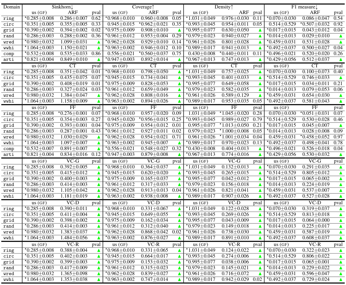
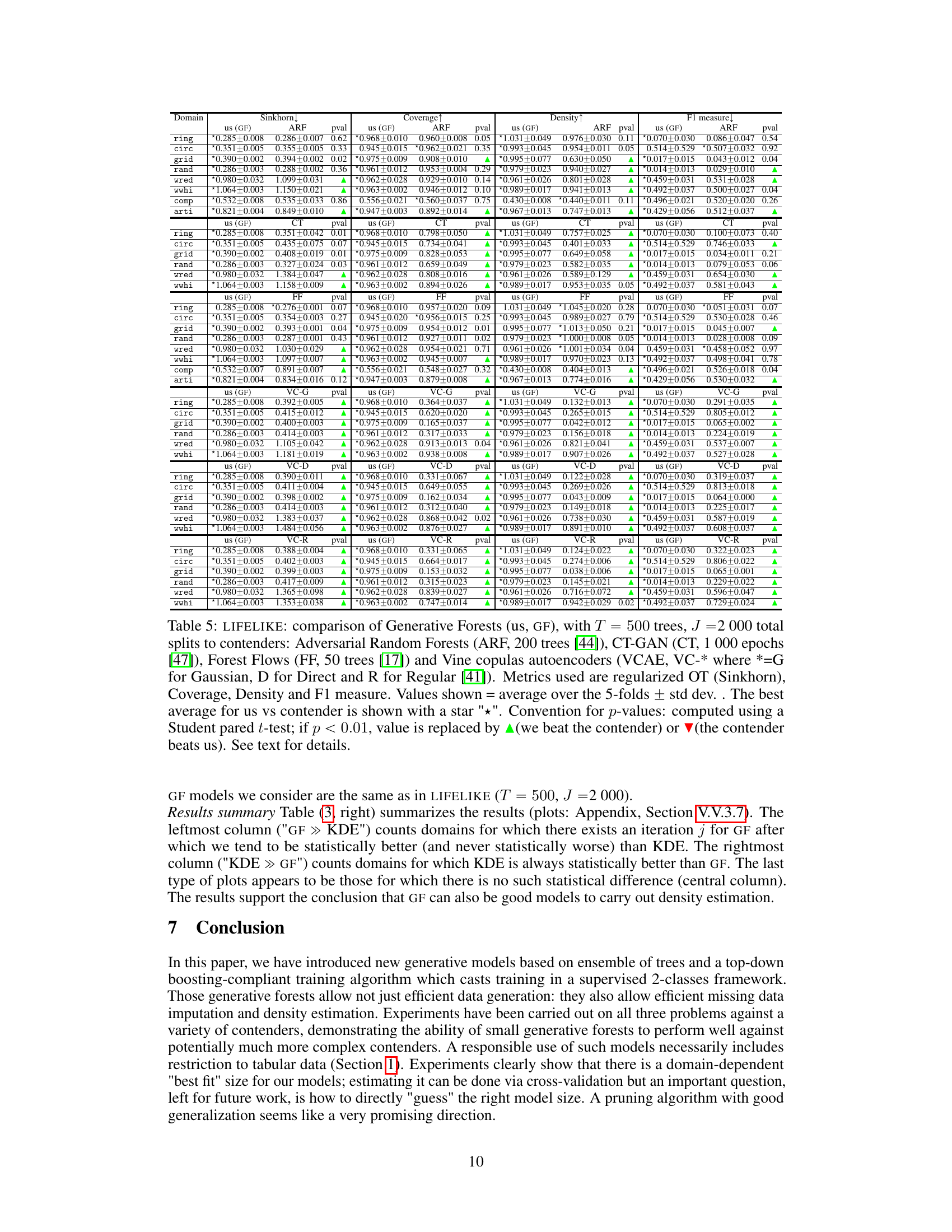
This table presents a comparison of the performance of Generative Forests against four other generative models on several datasets. The metrics used include Sinkhorn distance (a measure of the difference between probability distributions), coverage and density (measures of how well the generated data covers the real data), and the F1-score (a classification metric showing the accuracy of distinguishing between real and generated data). The results are averaged over 5-fold cross-validation, and the best-performing model for each metric is indicated with a star. P-values from paired t-tests indicate statistical significance of differences.

This table lists the 21 public and simulated datasets used in the experiments, including the source, size, number of categorical and numerical features, and presence of missing data. A tag is assigned to each dataset for easier referencing in other tables.

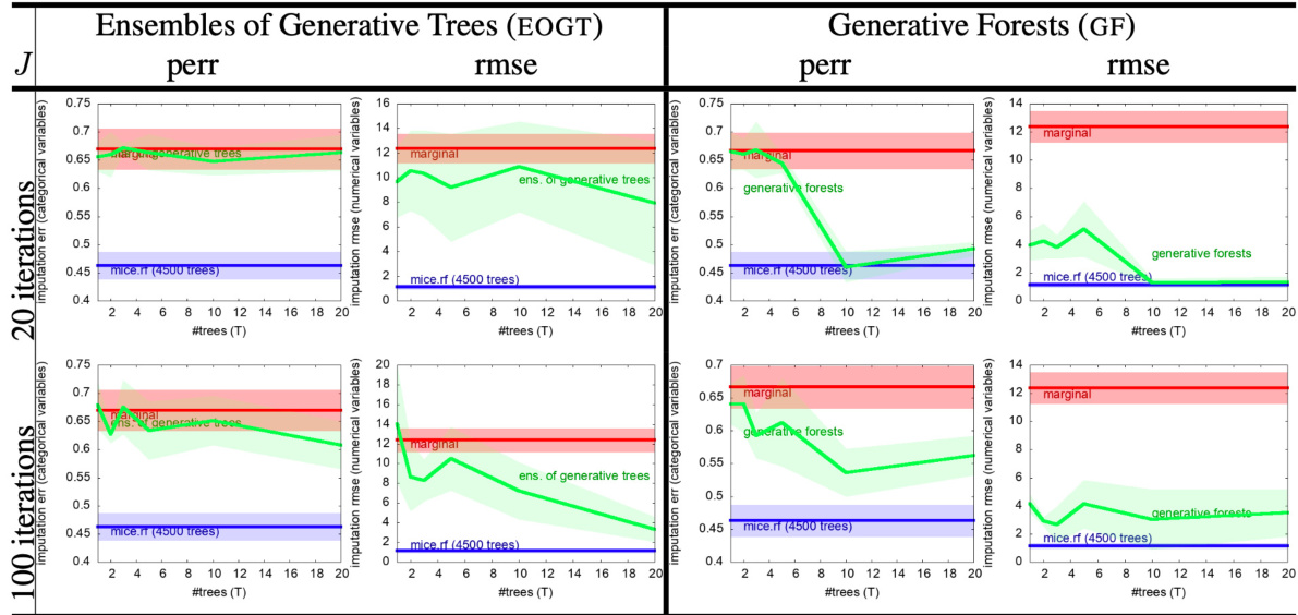
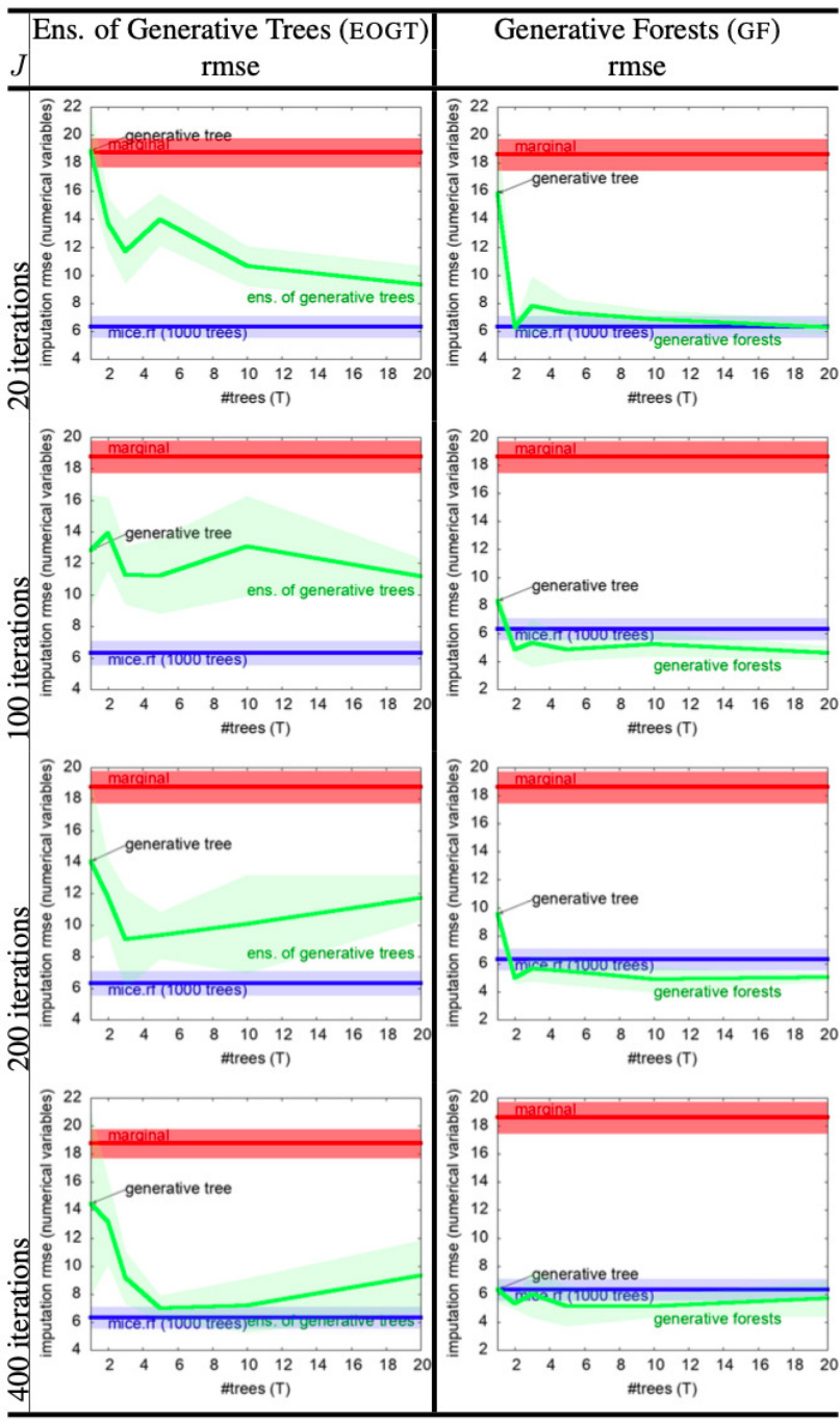
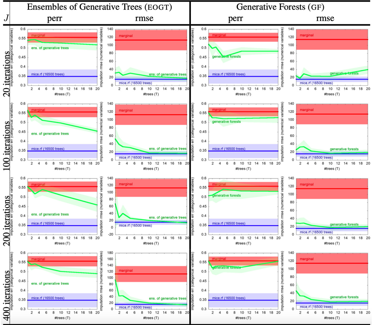
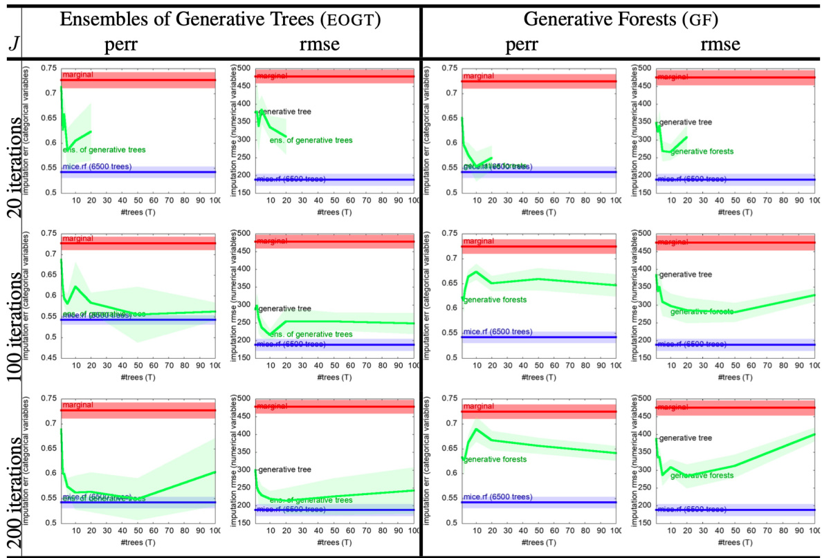
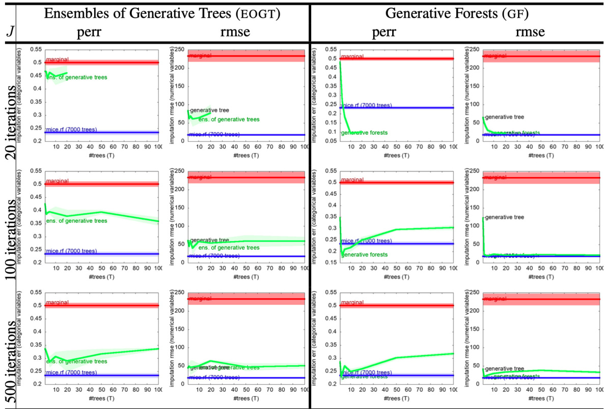
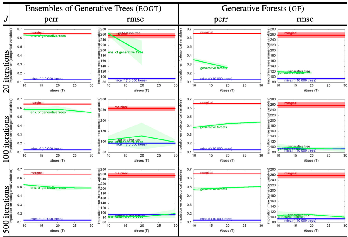
This table presents the results of missing data imputation experiments on two datasets, comparing the performance of Generative Forests (GF), MICE with random forests (MICE.RF), and a simple marginal imputation baseline. The results are displayed in terms of prediction error rate (perr) for categorical variables and root mean squared error (rmse) for numerical variables. The number of trees (T) in the GF model is varied, showing the effect on imputation accuracy.

This table lists the 21 public and simulated datasets used in the paper’s experiments. For each dataset, it provides the source, whether missing data was present, the total number of examples (m), the number of features (d), and a breakdown of categorical and numerical features. The table also includes a tag used to reference the dataset in subsequent tables.

This table lists the 21 public and simulated datasets used in the experiments. Each dataset is described by its name, a short tag, source, whether missing data is present, the number of examples (m), the number of features (d), and the count of categorical and numerical features.
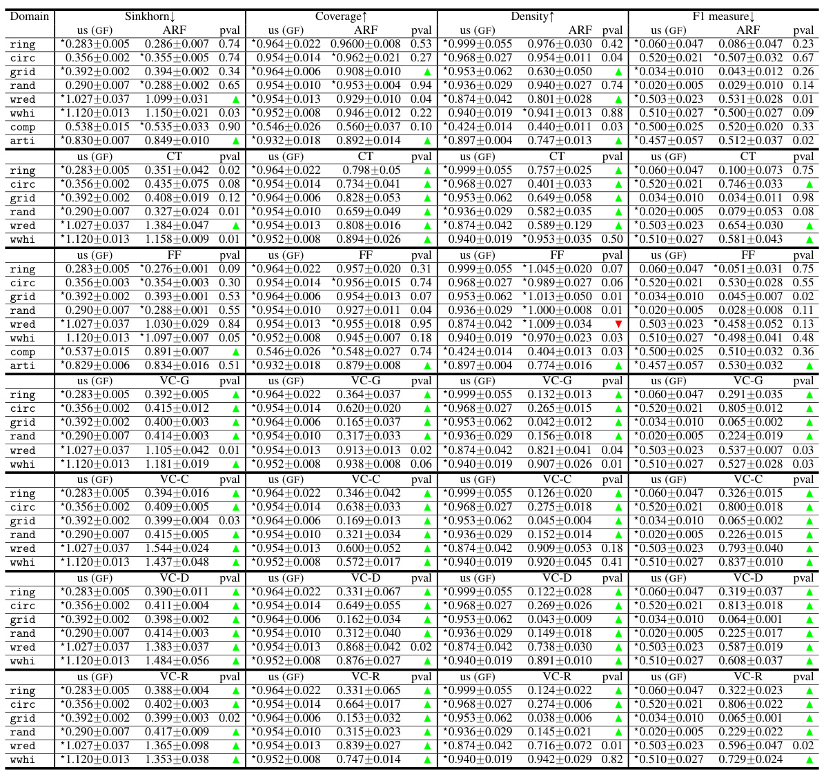
This table compares the performance of Generative Forests (GF) against four other generative models (ARF, CT-GAN, ForestFlow, and VCAE) across multiple datasets. The metrics used are Sinkhorn distance (a measure of distance between distributions), coverage, density, and F1 score. The results indicate the average performance across 5 folds of stratified cross validation, along with standard deviations. Statistically significant differences (p<0.01) between GF and the other methods are highlighted.

This table presents the results of the LIFELIKE experiment, comparing the performance of Generative Forests against several state-of-the-art generative models on various metrics such as Sinkhorn distance, coverage, density, and F1 measure. The results are averages over five stratified folds, with the best performance indicated by a star. P-values from paired t-tests indicate statistical significance.

This table compares the performance of Generative Forests against several state-of-the-art generative models on various datasets using four metrics: Sinkhorn distance, Coverage, Density, and F1 score. The p-values indicate statistical significance of the results, showing whether the Generative Forest outperforms the other models or vice-versa.

This table compares the performance of Generative Forests against four other generative models (ARF, CT-GAN, Forest Flows, and VCAE) across several datasets. The metrics used are Sinkhorn distance, coverage, density, and F1-score. The results show the average and standard deviation across 5-fold stratified cross-validation experiments. Statistically significant wins for Generative Forests are indicated using a star and p-values are provided.

This table compares the performance of Generative Forests against CT-GANs on various datasets. The Generative Forest model uses 500 trees and 2000 total splits. CT-GANs are trained with different numbers of epochs (10, 100, 300, 1000). The table shows the Sinkhorn distance, coverage, density and F1 measure for each model and dataset, along with p-values indicating statistical significance. Note that some CT-GAN runs crashed on certain folds, so the comparisons are restricted to the successful folds.
Full paper#
