TL;DR#
Many real-world machine learning applications require dealing with uncertainty in predictions, which standard point estimates fail to capture. Existing methods for quantifying predictive uncertainty often have limitations in terms of scalability or applicability to diverse model types. This necessitates more robust methods capable of generating accurate and reliable probabilistic forecasts.
The authors introduce Wasserstein Gradient Boosting (WGBoost), a novel algorithm that addresses these challenges. WGBoost leverages Wasserstein gradients to train weak learners on probability distributions. It is shown to achieve competitive performance on benchmark datasets across tasks such as classification and regression. WGBoost’s ability to produce non-parametric distributional predictions makes it particularly valuable for scenarios with high uncertainty and complex data patterns. The method is also applied to evidential learning to enhance its predictive uncertainty quantification.
Key Takeaways#
Why does it matter?#
This paper is important because it introduces a novel framework for distribution-valued supervised learning, a crucial area for handling uncertainty in machine learning predictions. This addresses the increasing need for probabilistic predictions in safety-critical applications and offers a new perspective on gradient boosting algorithms. The proposed method, Wasserstein Gradient Boosting (WGBoost), allows for non-parametric predictions of output distributions, which is especially relevant for dealing with complex real-world scenarios. The empirical results demonstrate the competitive performance of WGBoost across various real-world datasets.
Visual Insights#

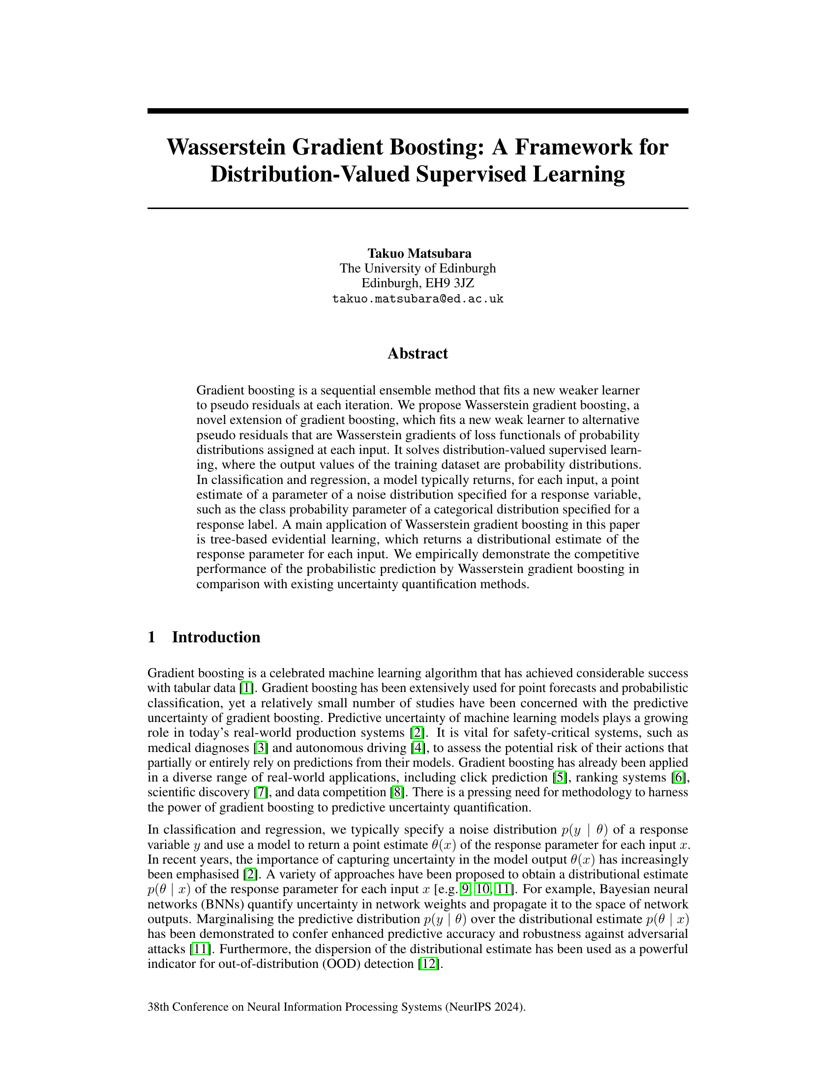
🔼 This figure shows the result of training the Wasserstein Gradient Boosting (WGBoost) model on a dataset with 10 input points and corresponding normal output distributions. Each subfigure represents the model’s performance after training with a different number of weak learners (0, 15, and 100). The blue shaded area shows the 95% highest probability density region of the true underlying function (sin(x)), while the red lines represent the 10 particles (approximations of the output distribution) generated by WGBoost for each input. As the number of weak learners increases, the red lines converge towards the true distribution, demonstrating the effectiveness of the model.
read the caption
Figure 1: Illustration of WGBoost trained on a set {xi, pi}101 whose inputs are 10 grid points in [-3.5, 3.5] and each output distribution is a normal distribution μi(θ) = N(θ | sin(xi), 0.5) over θ∈ R. The blue area indicates the 95% high probability region of the conditional distribution N(θ | sin(x), 0.5). WGBoost returns N = 10 particles (red lines) to predict the output distribution for each input x. This illustration uses the Gaussian kernel regressor for every weaker learner.
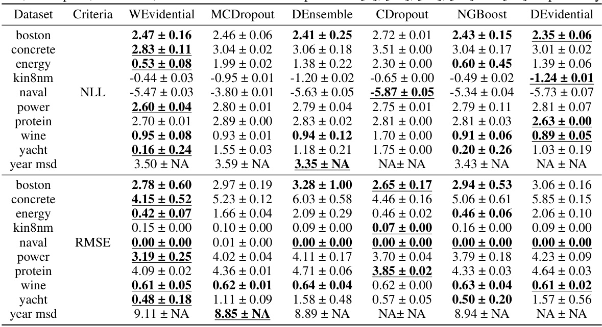
🔼 This table presents the negative log-likelihood (NLL) and root mean squared error (RMSE) for several regression datasets. It compares the performance of Wasserstein Gradient Boosting (WGBoost) against several other methods (MCDropout, Deep Ensemble, Concrete Dropout, NGBoost, and Deep Evidential Regression). The best result for each metric is underlined, and results within one standard deviation of the best are shown in bold. The results for the comparison methods are cited from other published works.
read the caption
Table 1: The NLLs and RMSEs for each dataset, where the best score is underlined and the scores whose standard deviation ranges include the best score are in bold. Results of MCDropout, DEnsembles, CDropout, NGBoost, and DEvidential were reported in [9], [10], [55], [32] and [13] respectively.
In-depth insights#
WGBoost Framework#
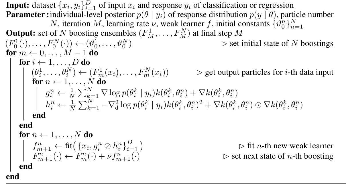
The Wasserstein Gradient Boosting (WGBoost) framework presents a novel approach to supervised learning by directly handling distribution-valued outputs. It extends traditional gradient boosting by leveraging Wasserstein gradients, which measure the optimal transport distance between probability distributions. This allows WGBoost to effectively learn models where the target variable is not a single point estimate but rather a probability distribution, offering a powerful way to model uncertainty. A key strength is its ability to handle nonparametric output distributions, unlike methods limited to specific closed-form distributions. The framework is particularly well-suited for evidential learning, where individual-level posterior distributions of parameters are used as targets, thus naturally incorporating uncertainty quantification. The use of particle approximations allows flexibility in representing complex distributions and avoids limitations associated with simpler parametric assumptions. The integration with tree-based weak learners makes WGBoost scalable and efficient, inheriting the strengths of well-established gradient boosting methods. However, challenges remain in estimating Wasserstein gradients accurately and efficiently, especially for high-dimensional data or complex distributions, highlighting areas for future research and potential improvements.
Evidential Learning#
Evidential learning presents a compelling paradigm shift in machine learning, moving beyond mere point predictions to encompass uncertainty quantification. Instead of providing a single output, evidential learning models yield probability distributions, offering a richer understanding of model confidence. This is particularly valuable in high-stakes applications such as medical diagnosis and autonomous driving where understanding uncertainty is crucial. A key strength lies in its ability to capture individual-level uncertainty, providing insights into the confidence of predictions for each data point. The integration with gradient boosting methods, as explored in Wasserstein Gradient Boosting, offers a powerful framework for building evidential models that leverage the efficiency and performance of established techniques. The use of Wasserstein gradient flows, a powerful concept in probability theory, enables the method to gracefully handle the complexity of probability distribution outputs. Overall, evidential learning holds significant promise for enhancing the reliability and trustworthiness of machine learning predictions, especially in safety-critical domains.
Wasserstein Gradient#
The concept of a Wasserstein gradient is crucial for understanding the core contribution of the research paper. It extends the typical gradient boosting approach by operating directly on probability distributions, not point estimates. This is achieved by using the Wasserstein gradient, which measures the change in a cost functional (like the KL divergence) as one probability distribution shifts towards another along the optimal transport path. This approach is especially relevant when dealing with distribution-valued supervised learning tasks, where the output is inherently uncertain and represented by a probability distribution rather than a single number. The Wasserstein gradient provides a way to calculate a direction of steepest descent in the space of probability distributions, which is used to guide the fitting of weak learners in a gradient boosting framework. The use of the Wasserstein distance ensures that the optimization is meaningful even when probability distributions have different support (different possible outcomes).
Real-World Datasets#
A dedicated section on ‘Real-World Datasets’ in a research paper would significantly strengthen the study’s credibility and impact. It should detail the selection criteria for choosing datasets, highlighting their relevance to the problem being addressed. Explicitly mentioning the source and characteristics (size, features, data types) of each dataset is crucial. Furthermore, a discussion on the potential biases or limitations inherent in real-world data, and how these were addressed or mitigated, would demonstrate a thorough understanding of the subject matter. Addressing the generalizability of findings to other datasets is vital to demonstrate robustness and broad applicability of the results, which strengthens the overall scientific rigor of the research. The results and performance metrics obtained from the various datasets should be meticulously documented and compared, showing the variability of results across different data distributions. This would paint a complete picture, enhancing transparency and fostering trust in the findings.
Future Research#
The ‘Future Research’ section of a research paper on Wasserstein Gradient Boosting (WGBoost) could explore several promising avenues. Extending WGBoost to handle non-tabular data is crucial, as the current framework is limited to tabular datasets. Investigating the convergence properties of WGBoost with different loss functionals and weak learners is vital for theoretical understanding and practical improvements. A comprehensive comparison with other uncertainty quantification methods should be conducted, particularly focusing on computational efficiency and the robustness of uncertainty estimates in various settings. Finally, exploring the applications of WGBoost in diverse domains beyond those explored in the paper—such as time series analysis, reinforcement learning, or causal inference—would significantly expand its impact and demonstrate its versatility. Addressing these aspects would enhance WGBoost’s applicability and provide more robust and accurate predictions in broader contexts.
More visual insights#
More on figures
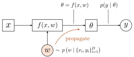
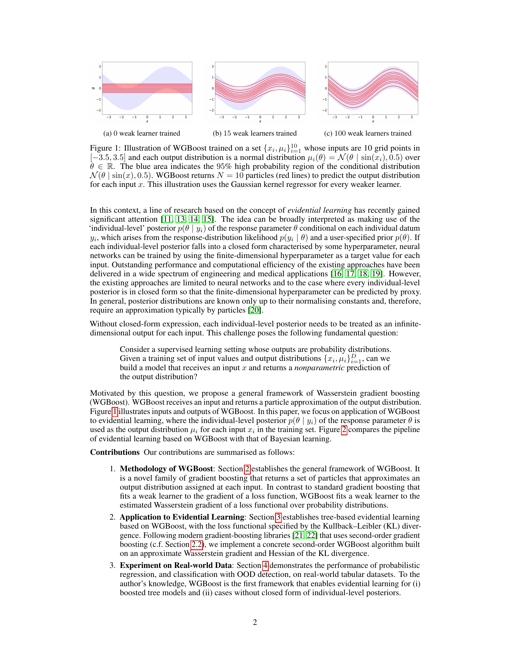
🔼 This figure compares Bayesian learning and evidential learning using WGBoost. Bayesian learning uses a global posterior distribution of model parameters to sample multiple models, while WGBoost uses individual-level posterior distributions as training outputs and returns particle approximations of the response parameter distribution for new inputs.
read the caption
Figure 2: Comparison of the pipeline of (a) Bayesian learning and (b) evidential learning based on WGBoost. The former uses the (global-level) posterior p(w | {xi, Yi}=1) of the model parameter w conditional on all data, and samples multiple models from it. The latter uses the individual-level posterior p(0 | yi) of the response parameter 0 as the output distribution of the training set, and trains WGBoost that returns a particle-based distributional estimate p(0 | x) of 0 for each input x.
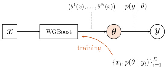
🔼 This figure compares Bayesian learning and evidential learning using WGBoost. Bayesian learning uses the global posterior distribution of model parameters to sample multiple models, while evidential learning leverages individual-level posterior distributions of response parameters as training outputs for WGBoost, resulting in a particle-based estimate of the response parameter’s distribution for new inputs.
read the caption
Figure 2: Comparison of the pipeline of (a) Bayesian learning and (b) evidential learning based on WGBoost. The former uses the (global-level) posterior p(w | {xi, Yi}=1) of the model parameter w conditional on all data, and samples multiple models from it. The latter uses the individual-level posterior p(0 | yi) of the response parameter 0 as the output distribution of the training set, and trains WGBoost that returns a particle-based distributional estimate p(0 | x) of 0 for each input x.
🔼 This figure illustrates how Wasserstein Gradient Boosting (WGBoost) works. It shows the output distribution learned by WGBoost for a simple dataset where inputs are 10 points along the x-axis, and each input is associated with a normal distribution as its output. The blue shaded area represents the 95% confidence interval of the true distribution, while the red lines represent particle approximations of the learned output distribution generated by WGBoost. The figure demonstrates how WGBoost improves its approximation of the true distribution as more weak learners are added (panels a-c).
read the caption
Figure 1: Illustration of WGBoost trained on a set {xi, pi}101 whose inputs are 10 grid points in [-3.5, 3.5] and each output distribution is a normal distribution μi(θ) = N(θ | sin(xi), 0.5) over θ∈ R. The blue area indicates the 95% high probability region of the conditional distribution N(θ | sin(x), 0.5). WGBoost returns N = 10 particles (red lines) to predict the output distribution for each input x. This illustration uses the Gaussian kernel regressor for every weaker learner.

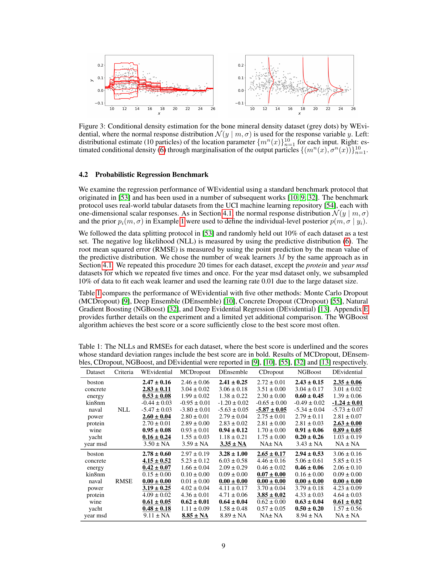
🔼 This figure shows the conditional density estimation results for the bone mineral density dataset using the WEvidential method. The left panel displays the distributional estimates (10 particles) of the location parameter for each input x. The right panel illustrates the estimated conditional density obtained by marginalizing over the output particles. Grey dots represent the actual data.
read the caption
Figure 3: Conditional density estimation for the bone mineral density dataset (grey dots) by WEvidential, where the normal response distribution N(y | m, σ) is used for the response variable y. Left: distributional estimate (10 particles) of the location parameter {mn(x)}n=110 for each input. Right: estimated conditional density (6) through marginalisation of the output particles {(mn(x), σn(x))}n=110.

🔼 This figure shows examples of output distributions generated by the WEvidential model for both in-distribution (non-OOD) and out-of-distribution (OOD) inputs. The left panel displays the output for a non-OOD sample belonging to class 4. The right panel shows the output for an OOD sample. In each panel, the red dots represent the individual particles generated by the model for each input. The shaded areas represent the kernel density estimation of the particle distributions. The difference in the spread and concentration of the particles for the in-distribution versus out-of-distribution sample highlights the model’s ability to capture and quantify uncertainty.
read the caption
Figure 4: Examples of the output particles (red dot) of WEvidential on the segment dataset, where the coloured area indicate the kernel density estimation of the output particles for each class.
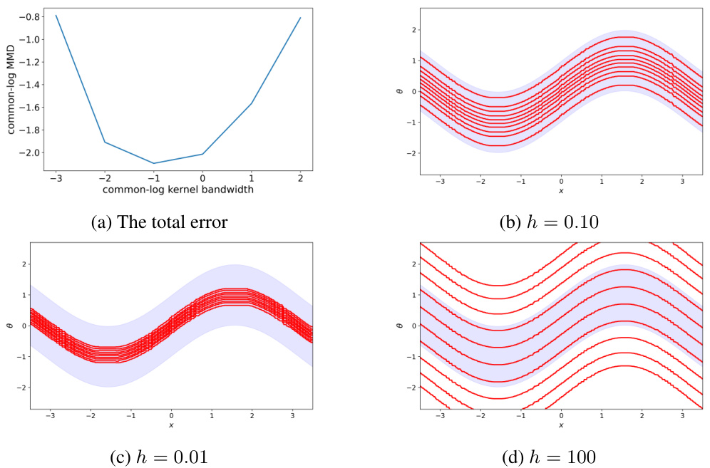
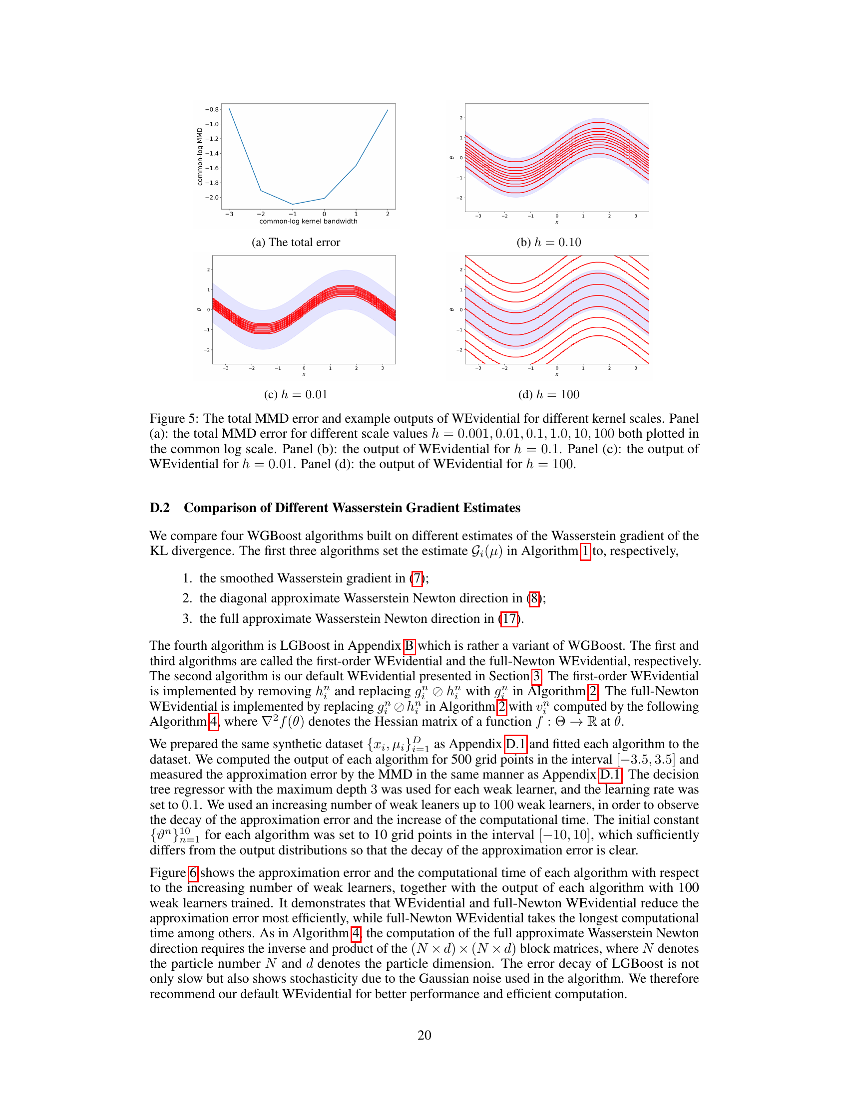
🔼 This figure shows the impact of the kernel bandwidth (h) on the performance of the WEvidential algorithm. Panel (a) presents the total MMD (Maximum Mean Discrepancy) error, a measure of the approximation error, across different bandwidths. Panels (b), (c), and (d) show example outputs of WEvidential using the three selected kernel bandwidths (h=0.10, h=0.01, and h=100), visually demonstrating the effect of the kernel choice on the algorithm’s prediction of the conditional density.
read the caption
Figure 5: The total MMD error and example outputs of WEvidential for different kernel scales. Panel (a): the total MMD error for different scale values h = 0.001, 0.01, 0.1, 1.0, 10, 100 both plotted in the common log scale. Panel (b): the output of WEvidential for h = 0.1. Panel (c): the output of WEvidential for h = 0.01. Panel (d): the output of WEvidential for h = 100.
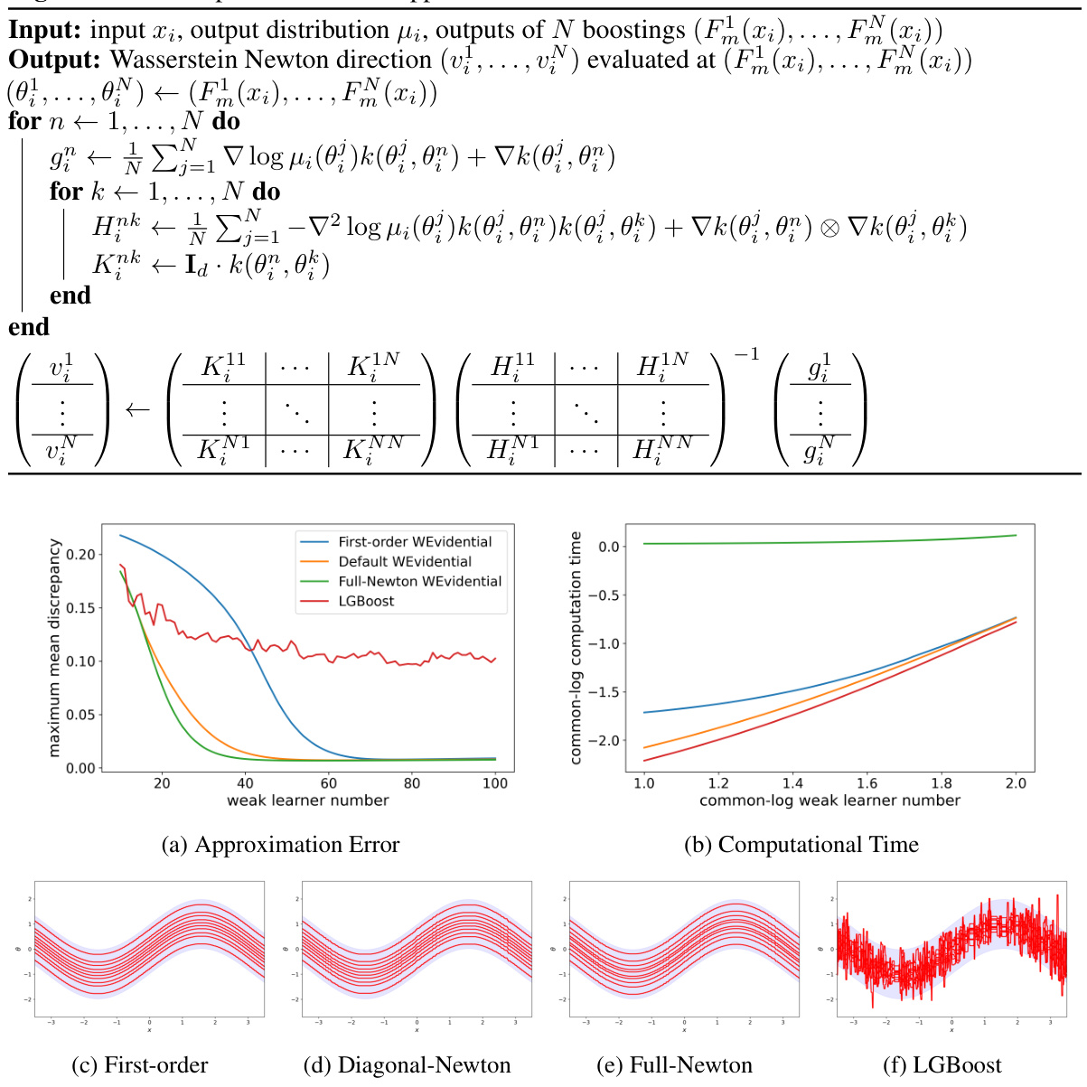
🔼 This figure compares four different WGBoost algorithms based on different Wasserstein gradient estimates. Panel (a) shows the approximation error (measured by Maximum Mean Discrepancy or MMD) versus the number of weak learners. Panel (b) shows the computation time versus the number of weak learners. Panels (c) through (f) display the output of each algorithm with 100 weak learners trained.
read the caption
Figure 6: The approximation error and computational time of the four different WGBoost algorithms. Panel (a): the approximation error of each algorithm measured by the MMD averaged over the inputs with respect to the number of weak learners. Panel (b): the computational time with respect to the number of weak learners in common logarithm scale. Panel (c)-(f): the outputs of the four algorithms each with 100 weak learners used.

🔼 This figure shows the results of applying the WEvidential algorithm to the bone mineral density dataset. The left panel displays the estimated location parameter for each input x as a distribution of 10 particles, while the right panel illustrates the resulting marginal conditional density obtained by integrating over these particles.
read the caption
Figure 3: Conditional density estimation for the bone mineral density dataset (grey dots) by WEvidential, where the normal response distribution N(y | m, σ) is used for the response variable y. Left: distributional estimate (10 particles) of the location parameter {mn(x)}n=110 for each input. Right: estimated conditional density (6) through marginalisation of the output particles {(mn(x), σn(x))}n=110.
More on tables

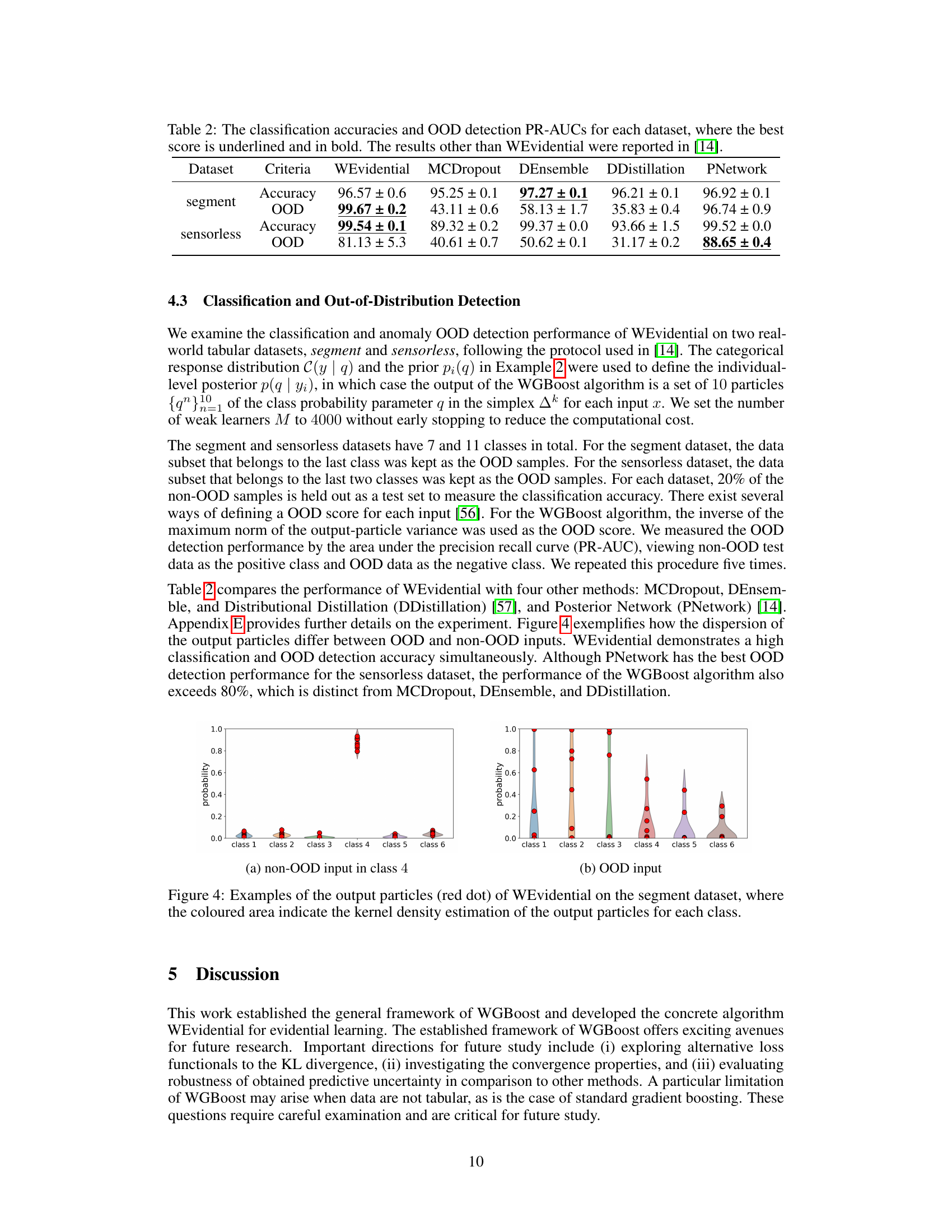
🔼 This table presents the classification accuracy and out-of-distribution (OOD) detection performance (measured by the area under the precision-recall curve, PR-AUC) of the proposed Wasserstein Gradient Boosting (WGBoost) algorithm and four other methods (MCDropout, DEnsemble, DDistillation, and PNetwork) on two real-world datasets (segment and sensorless). The best performance for each metric is highlighted in bold and underlined.
read the caption
Table 2: The classification accuracies and OOD detection PR-AUCs for each dataset, where the best score is underlined and in bold. The results other than WEvidential were reported in [14].

🔼 This table compares the performance of the proposed WEvidential model against five other probabilistic regression methods (MCDropout, Deep Ensemble, Concrete Dropout, Natural Gradient Boosting, and Deep Evidential Regression) across eight benchmark datasets. The results are presented in terms of the negative log-likelihood (NLL) and root mean squared error (RMSE), two common metrics used to evaluate the performance of regression models. The best performing model for each metric and dataset is underlined, and models with standard deviations that overlap the best score are shown in bold.
read the caption
Table 1: The NLLs and RMSEs for each dataset, where the best score is underlined and the scores whose standard deviation ranges include the best score are in bold. Results of MCDropout, DEnsembles, CDropout, NGBoost, and DEvidential were reported in [9], [10], [55], [32] and [13] respectively.
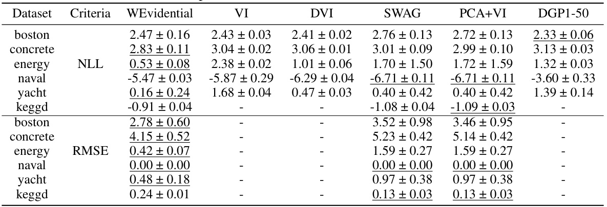
🔼 This table compares the negative log-likelihood (NLL) and root mean squared error (RMSE) of WEvidential against five other probabilistic regression methods across various datasets. The best performing method for each metric on each dataset is highlighted.
read the caption
Table 1: The NLLs and RMSEs for each dataset, where the best score is underlined and the scores whose standard deviation ranges include the best score are in bold. Results of MCDropout, DEnsembles, CDropout, NGBoost, and DEvidential were reported in [9], [10], [55], [32] and [13] respectively.

🔼 This table compares the out-of-distribution (OOD) detection performance of three different algorithms: WEvidential, NGBoost, and Random Forest (RForest), on the
segmentdataset. WEvidential is evaluated twice, once using its standard OOD metric and again using entropy as an alternative. The results show the accuracy and OOD detection performance (PR-AUC) for each algorithm. The goal is to assess which algorithm best identifies out-of-distribution samples.read the caption
Table 5: The OOD detection performance of WEvidential, NGBoost, and RForest on the segment dataset, where WEvidential (Entropy) indicates the result of WEvidential based on the entropy.

🔼 This table presents the results of a simulation study on a synthetic dataset to evaluate the performance of the WEvidential algorithm with varying learning rates. The number of weak learners was kept constant at 4000. The table shows the classification accuracy and out-of-distribution (OOD) detection performance (measured by the area under the precision-recall curve, or PR-AUC) for each learning rate.
read the caption
Table 6: The classification accuracy and OOD detection performance of WEvidential on the synthetic dataset for different learning rates, where the number of weak learners is fixed to 4000.

🔼 This table presents the results of a simulation study conducted to evaluate the impact of the number of weak learners on the performance of the WEvidential algorithm. The study used a synthetic dataset and varied the number of weak learners while keeping the learning rate constant at 0.4. The table shows that increasing the number of weak learners improves classification accuracy, but the effect on OOD detection performance is less clear.
read the caption
Table 7: The classification accuracy and OOD detection performance of WEvidential on the synthetic dataset for different numbers of weak learners, where the learning rate is fixed to 0.4.
Full paper#
