TL;DR#
Federated learning (FL) faces challenges due to high communication and computation costs, especially on resource-limited devices. Existing approaches for reducing these costs often involve sacrificing accuracy or introducing substantial computational overhead. This paper introduces SpaFL, a novel FL framework designed to mitigate these issues.
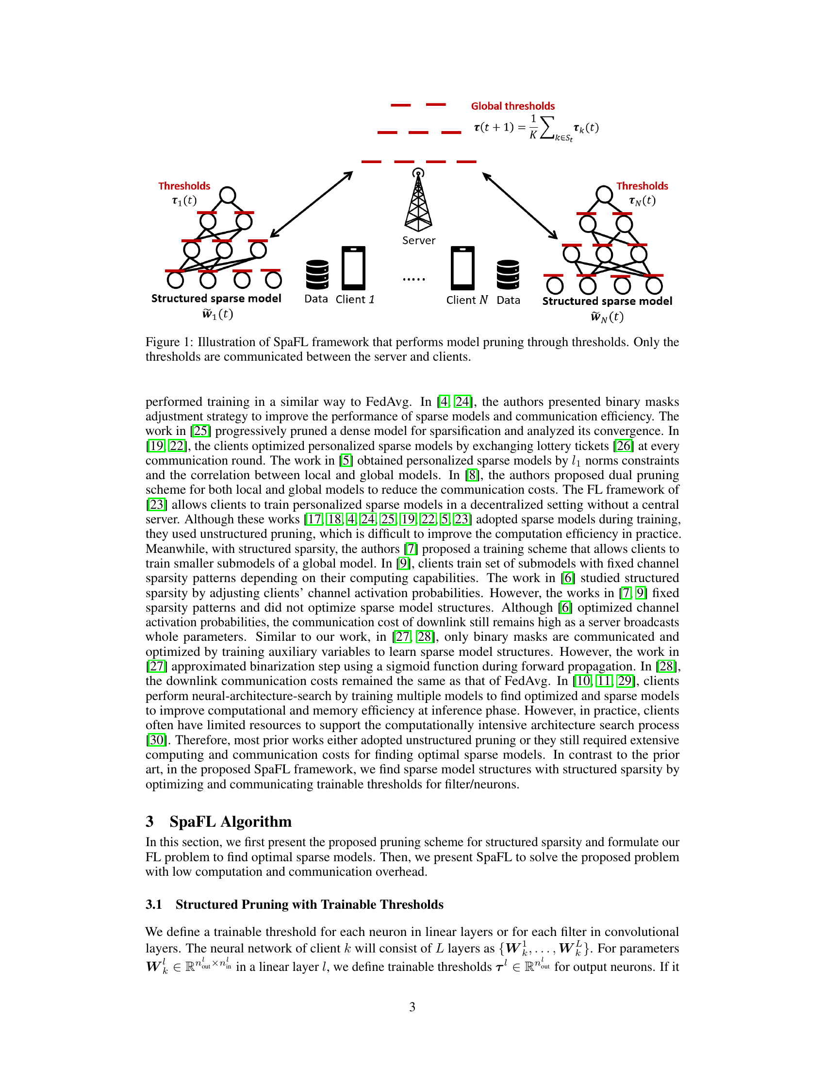
SpaFL employs a structured pruning technique using trainable thresholds to create sparse models efficiently. Only these thresholds are communicated between the server and clients, significantly reducing communication overhead. The method also optimizes the pruning process by updating model parameters based on aggregated parameter importance derived from global thresholds. Experimental results demonstrate that SpaFL significantly improves accuracy and reduces communication and computation costs compared to existing sparse FL baselines, making it a promising solution for real-world FL deployments.
Key Takeaways#
Why does it matter?#
This paper is important because it addresses the critical challenge of high communication and computational overhead in federated learning (FL). By proposing a novel communication-efficient FL framework (SpaFL) that optimizes sparse model structures with low computational overhead, it opens up new avenues for deploying FL in resource-constrained environments. The theoretical analysis and experimental results demonstrate SpaFL’s effectiveness, making it a significant contribution to the field. The code availability further enhances its impact.
Visual Insights#

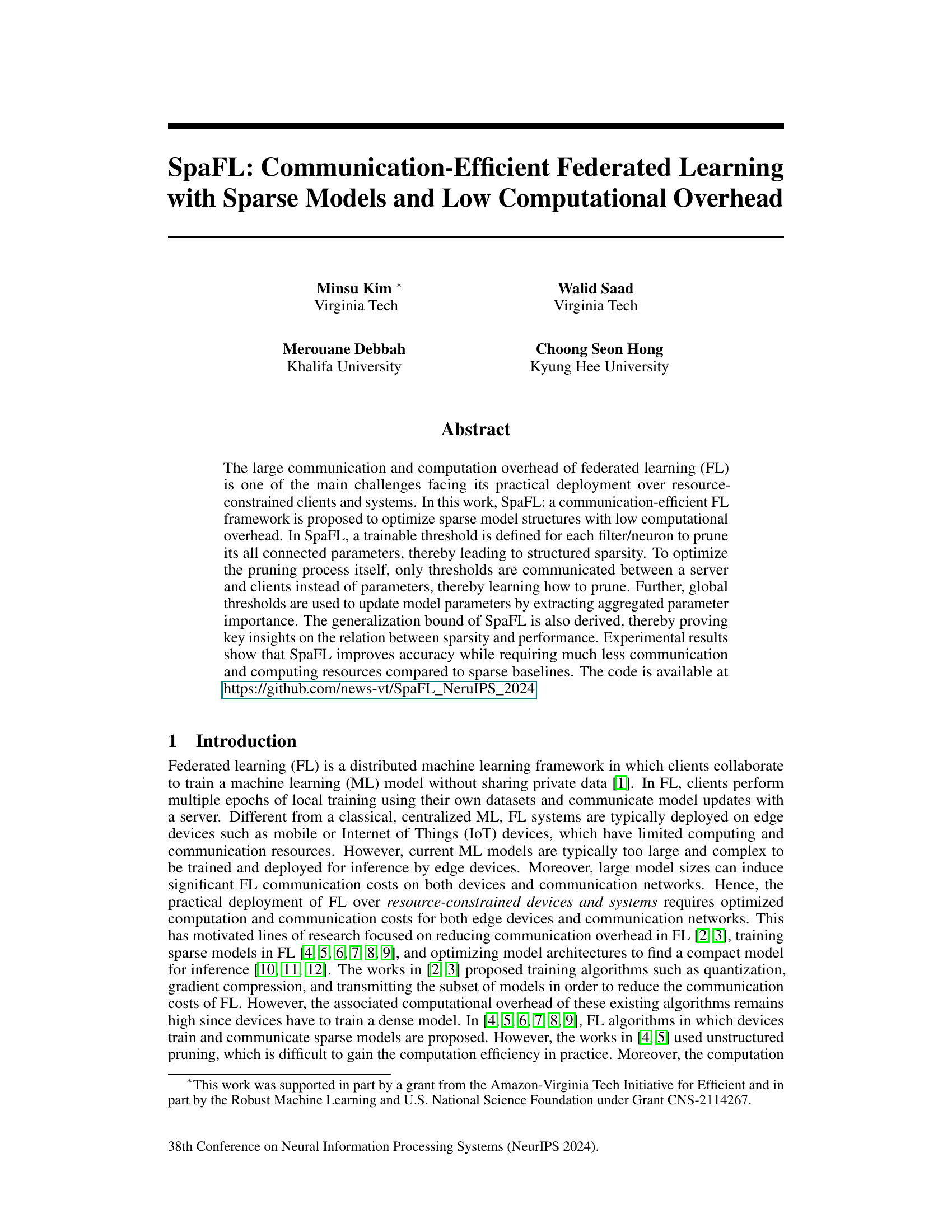
🔼 The figure illustrates the SpaFL framework, showing how trainable thresholds are used for structured pruning in a federated learning setting. Each client has a structured sparse model with individual thresholds for each filter/neuron. Only these thresholds, not the model parameters themselves, are communicated between the clients and the central server. The server aggregates the thresholds to produce global thresholds, which are then sent back to the clients for the next round of training. This process allows for efficient communication and personalized model pruning.
read the caption
Figure 1: Illustration of SpaFL framework that performs model pruning through thresholds. Only the thresholds are communicated between the server and clients.

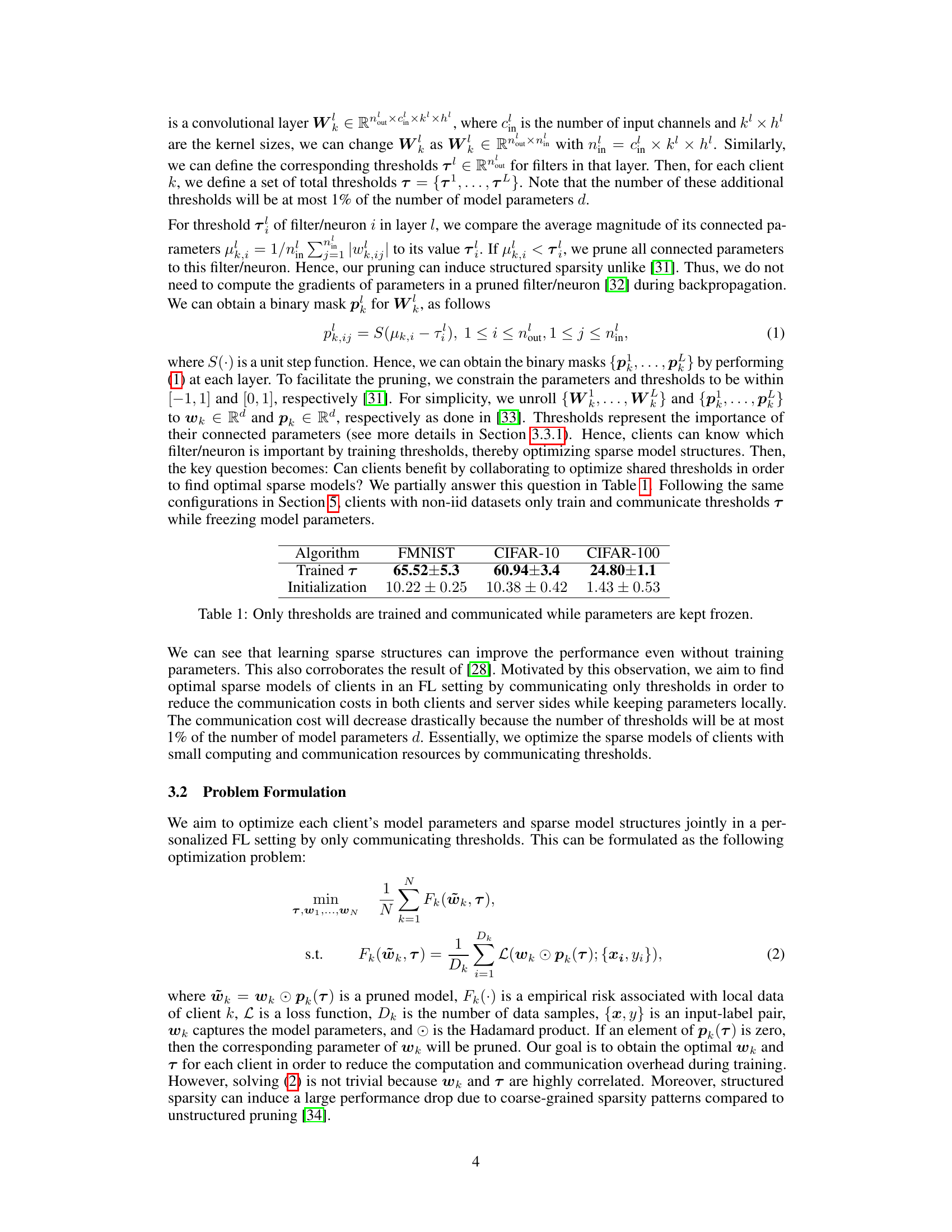
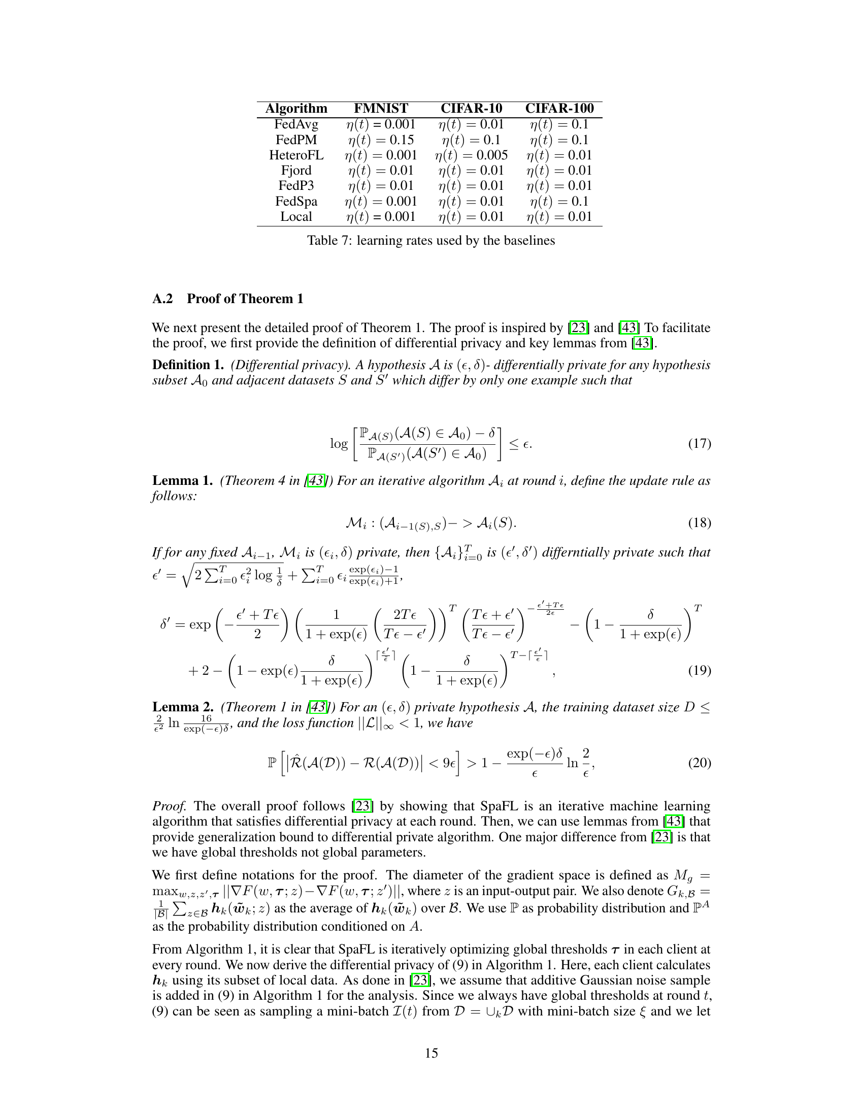
🔼 This table shows the results of an experiment where only the thresholds were trained and communicated, while the model parameters were kept frozen. The experiment was conducted on three datasets (FMNIST, CIFAR-10, and CIFAR-100). The table shows that even without training the model parameters, learning sparse structures through training only the thresholds, improves performance. The accuracy achieved by training thresholds alone is reported, along with the initial values of the thresholds used before training.
read the caption
Table 1: Only thresholds are trained and communicated while parameters are kept frozen.
In-depth insights#
SpaFL Framework#
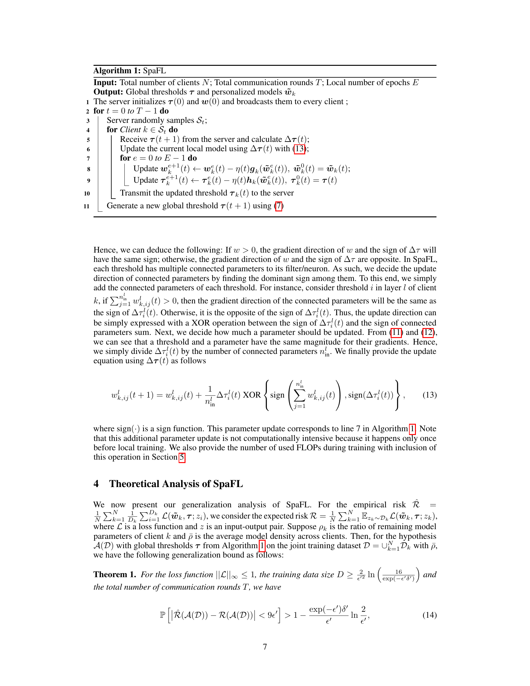
The SpaFL framework, designed for communication-efficient federated learning, presents a novel approach to optimize sparse model structures while minimizing computational overhead. Central to SpaFL is the use of trainable thresholds, one for each filter/neuron, to prune connected parameters, achieving structured sparsity. Unlike methods communicating entire parameters, SpaFL only shares thresholds between clients and server, significantly reducing communication costs. This allows for personalized sparse models on individual clients while leveraging global information through aggregated parameter importance. The theoretical analysis of SpaFL includes a generalization bound, demonstrating the relationship between sparsity and performance. Experimental results showcase SpaFL’s efficiency, achieving improved accuracy with substantially reduced communication and computation resources compared to existing dense and sparse baselines. This makes SpaFL particularly attractive for resource-constrained FL deployments.
Threshold Training#
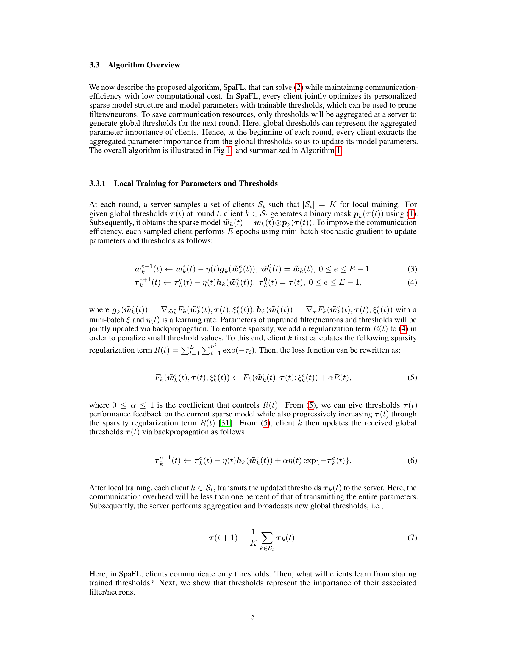
Threshold training is a novel approach to training sparse neural networks by introducing a trainable threshold for each neuron or filter. This threshold determines whether the connected parameters are pruned, leading to structured sparsity. The key advantage is that only thresholds, not parameters, need to be communicated, drastically reducing communication overhead in federated learning. Global thresholds, aggregated from individual client thresholds, guide the pruning process across devices. This technique allows each client to learn how to prune its model most efficiently, leading to personalized sparse models that improve accuracy and efficiency compared to traditional sparse methods. The impact on generalization is also investigated, highlighting the relationship between sparsity and performance.
Communication Efficiency#
The paper focuses on improving communication efficiency in federated learning (FL). Reducing communication overhead is crucial for practical FL, especially in resource-constrained environments. The core idea is to leverage sparse model structures and transmit only essential information between clients and the server. This is achieved by using trainable thresholds to prune model parameters, resulting in significantly less data transmission. The use of trainable thresholds allows the model to learn optimal sparsity patterns, improving accuracy while minimizing communication costs. Theoretical analysis supports the effectiveness of the approach by showing a relationship between sparsity and generalization performance. Experimental results demonstrate that the proposed method substantially outperforms baselines in terms of communication efficiency and accuracy, highlighting its practical potential for deploying FL in real-world settings.
Generalization Bound#
A generalization bound in machine learning provides a theoretical guarantee on the difference between a model’s performance on training data and its performance on unseen data. For federated learning (FL), where data is distributed across multiple clients, establishing a tight generalization bound is crucial, as it provides confidence in the model’s ability to generalize to new, unseen data from various clients. The complexity of FL, involving local training, communication rounds, and heterogeneous data distributions, makes deriving such a bound challenging. A well-crafted generalization bound often depends on factors like the number of clients, the data heterogeneity among clients, and the model’s sparsity (if applicable). A strong generalization bound suggests better performance and robustness. Conversely, a loose or non-existent bound raises concerns about the model’s reliability in real-world scenarios and highlights the need for improved theoretical understanding and model development. In the context of sparse FL models, the generalization bound might reveal interesting relationships between sparsity, communication efficiency, and the model’s generalization ability, potentially offering guidelines for designing communication-efficient and robust models.
Future of SpaFL#
The future of SpaFL hinges on addressing its current limitations and exploring new avenues for improvement. Reducing the computational overhead further is crucial, perhaps through more efficient threshold optimization algorithms or hardware acceleration. Investigating different sparsity patterns and pruning strategies beyond the structured approach could unlock further performance gains. Theoretical analysis needs expansion to provide tighter generalization bounds and encompass scenarios with non-i.i.d. data and varying levels of client participation. Extending SpaFL to support various model architectures beyond CNNs and ViTs, such as transformers or graph neural networks, would broaden its applicability. Finally, research into the robustness of SpaFL against adversarial attacks and its privacy implications in more complex settings is vital for real-world deployment.
More visual insights#
More on figures

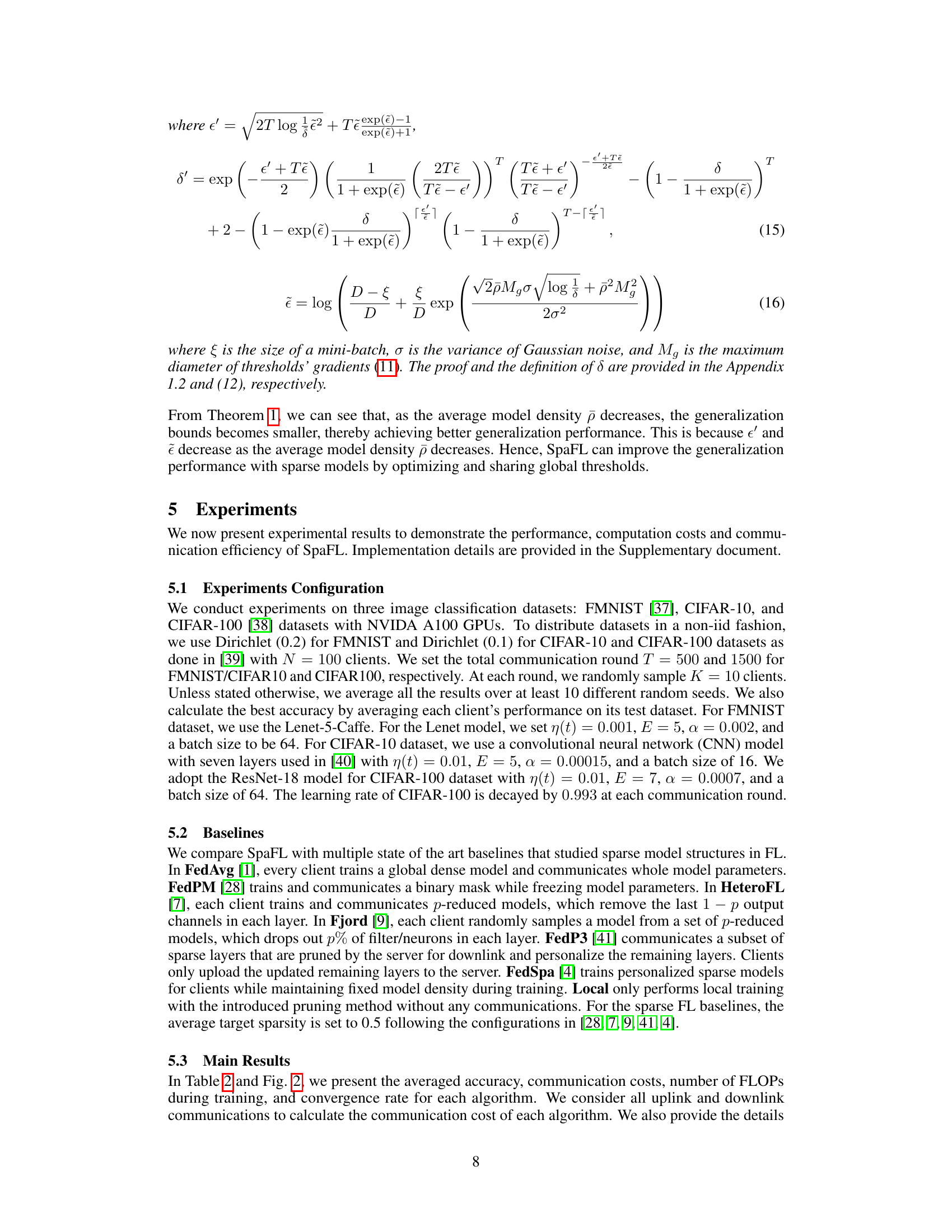
🔼 This figure shows the learning curves of SpaFL and several baseline algorithms on three image classification datasets: FMNIST, CIFAR-10, and CIFAR-100. The x-axis represents the number of communication rounds, and the y-axis represents the accuracy achieved. The plot visually compares the training performance and convergence speed of SpaFL against other approaches, illustrating its effectiveness in achieving high accuracy with fewer communication rounds.
read the caption
Figure 2: Learning curves on FMNIST, CIFAR-10, and CIFAR-100

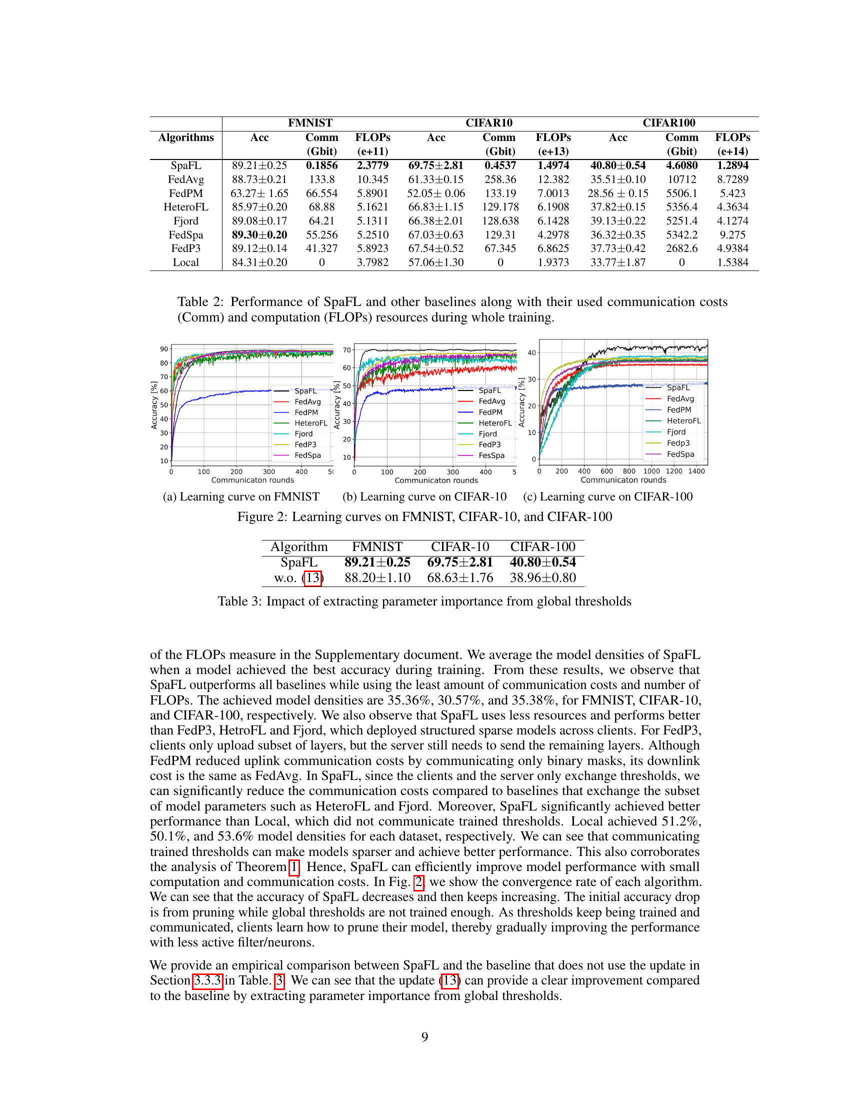
🔼 This figure visualizes the sparsity patterns of the first convolutional layer (conv1) in a model trained on the CIFAR-10 dataset across different training rounds (40, 150, and 500). Each subfigure represents a specific training round, showing a heatmap where black represents active filters/neurons and white represents pruned ones. The x-axis shows the different clients, and the y-axis represents the filters. This visualization demonstrates how SpaFL, the proposed algorithm, learns to optimize sparse model structures by evolving the sparsity patterns over the training process, indicating that initially many filters are pruned and then some are recovered as training progresses.
read the caption
Figure 3: Sparsity pattern of conv1 layer on CIFAR-10

🔼 This figure visualizes the sparsity patterns of the first convolutional layer (conv1) across different training rounds (40, 150, and 500) on the CIFAR-10 dataset. Each subplot represents a specific training round and shows the sparsity pattern for each client. Black pixels indicate active filters/neurons, while white pixels represent pruned (inactive) ones. The figure demonstrates how the sparsity patterns evolve as training progresses, showing that clients gradually learn common sparse model structures by optimizing shared thresholds across training rounds. Note that some filters initially pruned may be reactivated during the training process.
read the caption
Figure 3: Sparsity pattern of conv1 layer on CIFAR-10

🔼 This figure visualizes the sparsity patterns of the first convolutional layer (conv1) across different training rounds (40, 150, and 500) on the CIFAR-10 dataset. Each subfigure shows a heatmap where each row represents a client and each column represents a filter in the layer. Black indicates a filter that is active (not pruned) while white represents a pruned filter. The figure demonstrates how the sparsity pattern evolves during training. It shows how the sparsity patterns differ across clients, indicating personalization, and also how the overall sparsity changes over time.
read the caption
Figure 3: Sparsity pattern of conv1 layer on CIFAR-10

🔼 This figure shows the sparsity patterns of the first convolutional layer (conv1) with 64 filters and three input channels on the CIFAR-10 dataset at different communication rounds (40, 150, and 500). Active filters are shown in black, while pruned filters are shown in white. The figure illustrates how SpaFL enables clients to learn common, optimized sparse model structures across training rounds by optimizing thresholds. Initially (round 40), there is high sparsity. As training progresses, pruned filters may be recovered and sparsity is gradually enforced. This demonstrates the dynamic and adaptive nature of the sparsity patterns learned by the SpaFL algorithm.
read the caption
Figure 3: Sparsity pattern of conv1 layer on CIFAR-10
More on tables

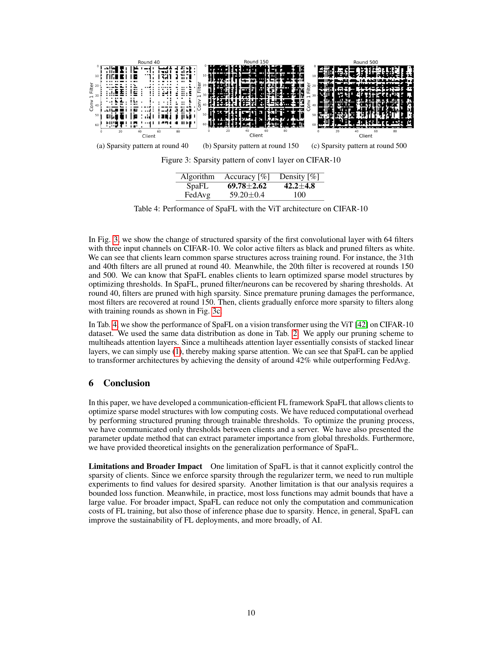
🔼 This table presents a comparison of SpaFL’s performance against several baseline federated learning algorithms across three benchmark datasets (FMNIST, CIFAR-10, and CIFAR-100). The metrics compared include accuracy, communication costs (in Gbits), and computational costs (in e+11, e+13, and e+14 FLOPs for the respective datasets). The table highlights SpaFL’s superior performance in terms of accuracy while significantly reducing communication and computational overhead compared to the baselines. This demonstrates the effectiveness of SpaFL in optimizing sparse models with low computational overhead.
read the caption
Table 2: Performance of SpaFL and other baselines along with their used communication costs (Comm) and computation (FLOPs) resources during whole training.

🔼 This table compares the performance of SpaFL against other federated learning algorithms across three datasets: FMNIST, CIFAR-10, and CIFAR-100. The metrics presented are the accuracy achieved, the amount of communication in gigabits, the number of floating point operations (FLOPs) in e+11, e+13, and e+14, respectively for each dataset. The results highlight SpaFL’s efficiency in achieving high accuracy while using significantly fewer communication and computational resources compared to the baselines.
read the caption
Table 2: Performance of SpaFL and other baselines along with their used communication costs (Comm) and computation (FLOPs) resources during whole training.

🔼 This table compares the performance of SpaFL and FedAvg on the CIFAR-10 dataset using the Vision Transformer (ViT) architecture. It shows that SpaFL achieves a significantly higher accuracy (69.78% ± 2.62%) compared to FedAvg (59.20% ± 0.4%), while maintaining a much sparser model (42.2% ± 4.8% density) compared to the dense model of FedAvg (100% density). This highlights SpaFL’s effectiveness in achieving high accuracy with low computational cost by optimizing sparse model structures.
read the caption
Table 4: Performance of SpaFL with the ViT architecture on CIFAR-10

🔼 This table compares the performance of SpaFL against other baseline methods (FedAvg, FedPM, HeteroFL, Fjord, FedSpa, FedP3, and Local) across three datasets: FMNIST, CIFAR-10, and CIFAR-100. For each method, it presents the accuracy achieved, the communication cost in gigabits (Gbit), and the number of floating-point operations (FLOPs) in e+11, e+13, and e+14, respectively. The results demonstrate SpaFL’s superior performance in terms of accuracy while maintaining significantly lower communication and computation costs.
read the caption
Table 2: Performance of SpaFL and other baselines along with their used communication costs (Comm) and computation (FLOPs) resources during whole training.
🔼 This table compares the performance of SpaFL against several other baseline algorithms across three datasets (FMNIST, CIFAR-10, and CIFAR-100). The metrics presented are accuracy, communication costs (in Gbits), FLOPs (floating point operations, a measure of computational cost in e+11, e+13, and e+14), and the model density (percentage of non-zero parameters). The table demonstrates SpaFL’s efficiency in achieving high accuracy with significantly reduced communication and computation resources compared to the baselines.
read the caption
Table 2: Performance of SpaFL and other baselines along with their used communication costs (Comm) and computation (FLOPs) resources during whole training.
Full paper#
