↗ OpenReview ↗ NeurIPS Homepage ↗ Chat
TL;DR#
Many real-world dynamical systems exhibit complex, nonlinear behavior, making them difficult to model using traditional methods. Neural Ordinary Differential Equations (NODEs) offer a promising approach due to their ability to handle continuous-time dynamics. However, existing NODEs often lack scalability and may struggle with guaranteeing convergence, particularly in highly complex scenarios. This is where the limitations arise and where this paper addresses the problem.
This paper introduces ControlSynth Neural ODEs (CSODEs), a new type of NODE architecture designed to overcome these limitations. CSODEs achieve guaranteed convergence through the use of tractable linear inequalities, making them more robust and reliable. The incorporation of an additional control term allows CSODEs to effectively capture dynamics at multiple scales simultaneously, greatly enhancing their flexibility and applicability to complex systems. Extensive experiments show that CSODEs outperform existing NODE variants, demonstrating significant improvements in accuracy and predictive performance across diverse challenging dynamical systems.
Key Takeaways#
Why does it matter?#
This paper is crucial for researchers in dynamical systems modeling, offering guaranteed convergence in highly nonlinear systems and opening avenues for improving the scalability and predictive ability of neural ODEs. Its tractable linear inequalities for convergence and the introduction of a control term for multi-scale dynamics make it highly relevant to current research trends in AI, physics, and engineering.
Visual Insights#

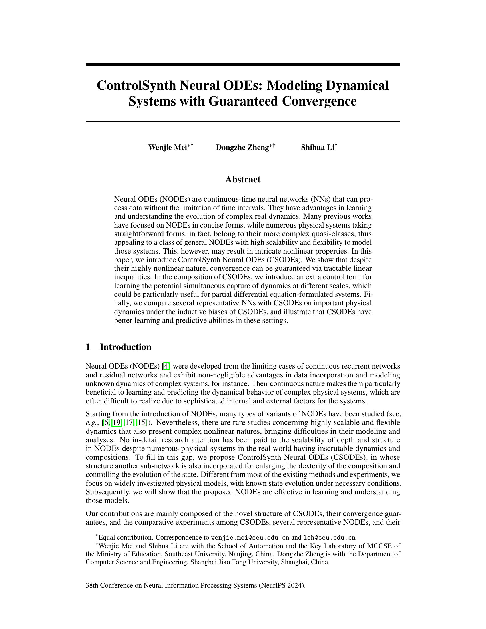
This figure illustrates the computational flow of the ControlSynth Neural ODEs (CSODEs) solver using the forward Euler method as an example. It shows how the control input (ut) and the state vector (xt) are updated at each time step (Δt) using a combination of neural networks (NNs) and matrix operations. Specifically, the control input is processed by the NN g(·), and the state vector is transformed by the NNs A1f1(W1·), …, Амƒм(Wм.) and the matrix A0. The outputs of these transformations are then combined and used to update the control input and the state vector for the next time step. The function h(·) represents the update neural function which handles the process of updating the variables using the results from the NNs and matrix operations.

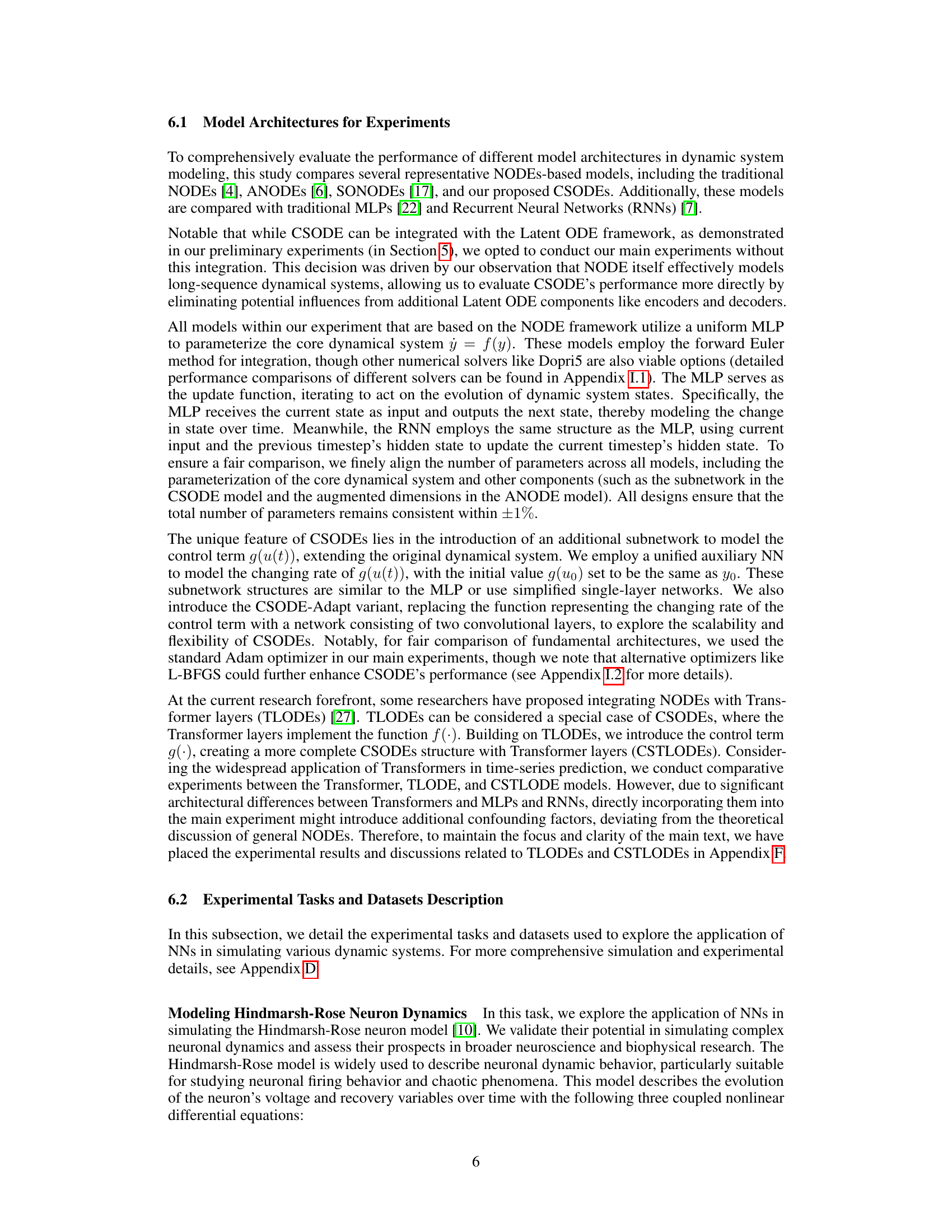
This table compares the performance of four different neural ordinary differential equation (NODE) based models (NODE, ANODE, SONODE, and CSODE) on the MNIST image classification task. The metrics used for comparison are test error rate, the number of parameters, floating-point operations per second (FLOPS), average batch processing time, and peak memory usage. The results show that while CSODE has slightly better performance than other models (0.39% test error rate), the computational cost is comparable across all four models.
In-depth insights#
CSODE: Convergence#
The heading ‘CSODE: Convergence’ suggests a section dedicated to proving the convergence properties of ControlSynth Neural Ordinary Differential Equations (CSODEs). A rigorous mathematical treatment is likely presented, demonstrating that under specific conditions (e.g., on activation functions, system parameters), the CSODE model’s solution will converge to a stable equilibrium. The proof likely involves constructing a Lyapunov function to show that the system’s energy decreases monotonically over time. Assumptions on the activation functions might be required to guarantee monotonicity and boundedness of the solutions. The analysis may explore different aspects of convergence, including global asymptotic stability, to provide a comprehensive understanding of CSODE’s behavior. The existence and uniqueness of solutions are likely addressed, alongside detailed conditions ensuring that CSODEs do not exhibit chaotic or divergent behavior. The section would ultimately establish the reliability and predictability of the CSODE model for various applications, which is crucial for its practical use in modeling dynamic systems.
ControlSynth NN#
ControlSynth Neural Networks (CSNNs) represent a novel architecture designed to enhance the capabilities of traditional neural networks, particularly in modeling complex dynamical systems. The core innovation lies in the integration of a control term within the network’s structure. This control mechanism allows for greater flexibility and scalability, enabling CSNNs to model systems with intricate nonlinearities and varying scales. A key advantage is the potential for guaranteed convergence, even in highly nonlinear scenarios. This is achieved through tractable linear inequalities, which provide a level of stability and predictability not typically found in standard neural networks. CSNNs demonstrate improved learning and predictive abilities compared to traditional methods across various benchmarks, suggesting their potential for use in diverse applications involving the modeling of complex physical or biological systems. Further research could focus on exploring the impact of different control strategies, as well as the development of tailored training algorithms to maximize the potential of this novel architecture.
Physical System Tests#
A hypothetical ‘Physical System Tests’ section in a research paper would likely involve evaluating the model’s performance on real-world or simulated physical systems. This could encompass diverse domains such as robotics, where the model controls a robot’s movement, fluid dynamics, where it predicts fluid flow, or chemical reactions, where it simulates chemical processes. The tests should focus on assessing the model’s ability to generalize to unseen data, handle noisy inputs, and make accurate predictions under various conditions. Quantitative metrics, such as mean squared error or R-squared, would be crucial for evaluating the model’s predictive accuracy. Qualitative analysis, comparing the model’s predictions to ground truth data visually, would provide further insights into its performance. Importantly, the choice of test systems and evaluation metrics should be justified, reflecting their relevance to the model’s application and ensuring a rigorous evaluation process. The use of both synthetic and real-world systems is also ideal to validate the robustness of the model.
Scalability & Limits#
A crucial aspect of evaluating any machine learning model is its scalability and inherent limitations. Scalability refers to the model’s ability to handle increasingly large datasets and complex tasks without significant performance degradation. Limits, on the other hand, represent the boundaries of the model’s capabilities, encompassing factors such as computational cost, memory requirements, and the model’s capacity to generalize to unseen data. In the context of neural ordinary differential equations (NODEs) and their variants, these factors are particularly important. NODEs’ continuous nature allows for more flexible modeling but also introduces challenges in terms of computational complexity. The model’s architecture, including the depth and width of the network, significantly influences both scalability and limits. Increasing the complexity might enhance predictive accuracy but also lead to higher computational costs and potential overfitting. Therefore, researchers need to consider a careful trade-off between enhancing model capabilities and maintaining computational feasibility. Furthermore, the ability of a model to generalize well to new, unseen data is crucial. Limits on generalization may arise from the model’s inherent inductive biases and its training data’s limitations. This highlights the need for careful consideration of dataset diversity and size during training.
Future Work#
The authors acknowledge limitations and suggest promising future research directions. Enhancing CSODE’s applicability to broader classes of dynamical systems is crucial, especially those exhibiting complex interactions and multi-scale phenomena. Improving the efficiency and scalability of CSODE’s training process is also vital, potentially through specialized algorithms or architectural modifications. Exploring the integration of CSODE with other advanced machine learning techniques such as transformers could unlock further improvements in model accuracy and predictive abilities. Investigating the sensitivity of CSODE to various hyperparameters and developing robust methods for tuning is essential for wider adoption. Finally, a deeper theoretical analysis could strengthen convergence guarantees and provide valuable insights into CSODE’s strengths and limitations. Rigorous empirical validation across a wider range of applications would also solidify CSODE’s position as a powerful tool for modeling dynamical systems.
More visual insights#
More on figures
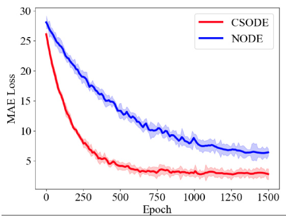
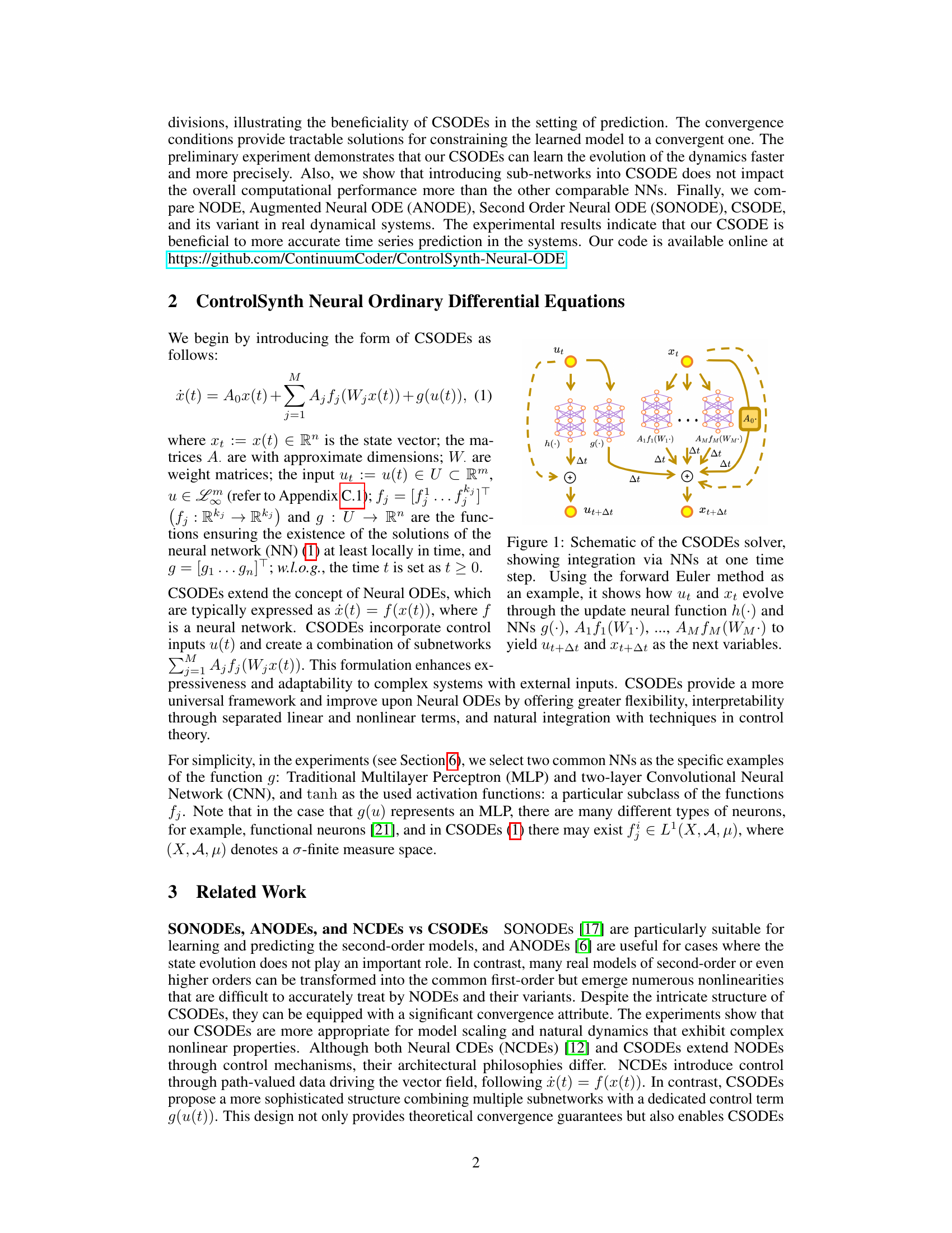
This figure shows the mean absolute error (MAE) loss curves for both the CSODE and NODE models during training. The x-axis represents the training epoch (iteration), and the y-axis shows the MAE loss. The CSODE model demonstrates faster convergence to a lower MAE loss compared to the NODE model, indicating improved learning efficiency and potentially better prediction accuracy.

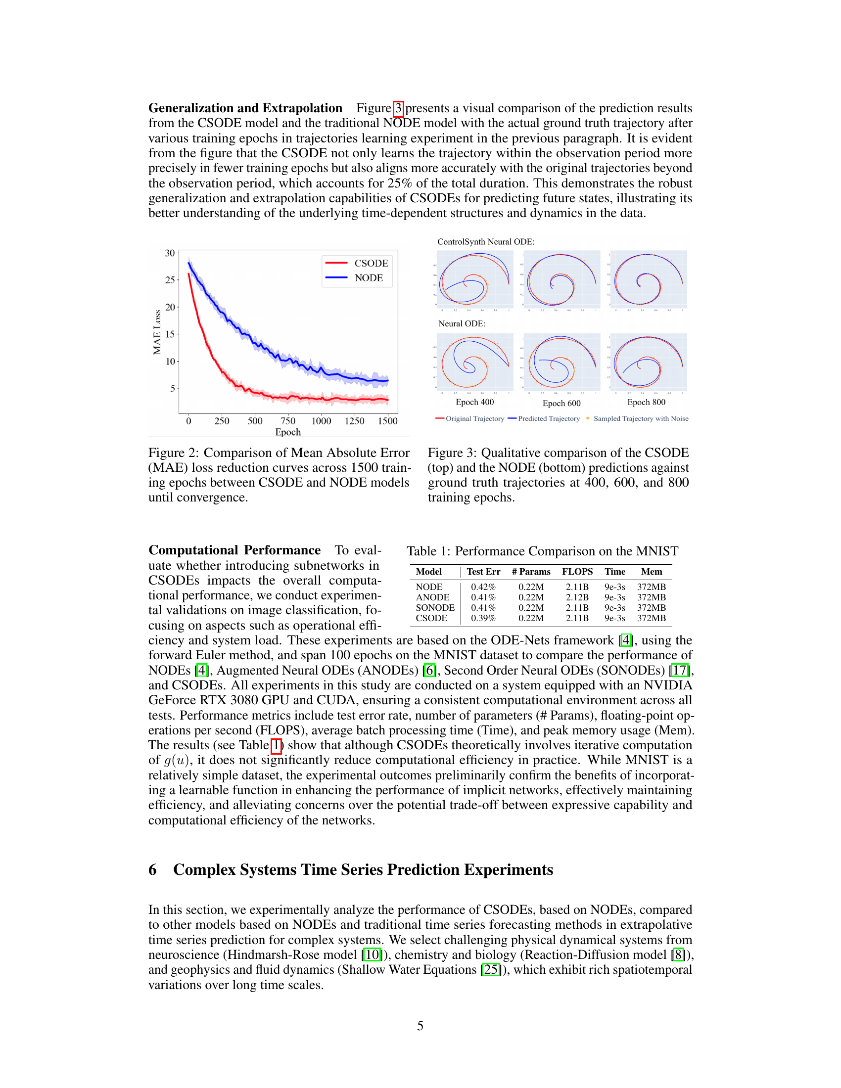
This figure compares the performance of CSODE and NODE models in learning and predicting spiral trajectories. The top row shows the results for CSODE, while the bottom row shows the results for NODE. Each column represents a different training epoch (400, 600, and 800). The orange dots represent the noisy sampled data points used for training, the red line represents the original trajectory, and the blue line represents the predicted trajectory from each model. The figure demonstrates that CSODE is able to learn the trajectory more accurately and generalize better than NODE.

This figure compares the prediction results of CSODE and NODE models against the actual ground truth trajectory at different training epochs (400, 600, and 800). It visually demonstrates that CSODE model achieves higher prediction accuracy and better aligns with the original trajectories compared to the NODE model, especially beyond the observation period. This showcases the superior generalization and extrapolation capabilities of CSODEs for predicting future states.
This figure compares the performance of CSODE and NODE models in predicting trajectories. It shows the predicted trajectories for both models alongside the true trajectory at three different training epochs (400, 600, and 800). This allows for a visual assessment of how well each model learns and generalizes over time, and highlights the superior performance of CSODE, which is much closer to the ground truth, especially at later epochs. The sampled trajectory with noise illustrates the robustness of the models in the presence of noise.

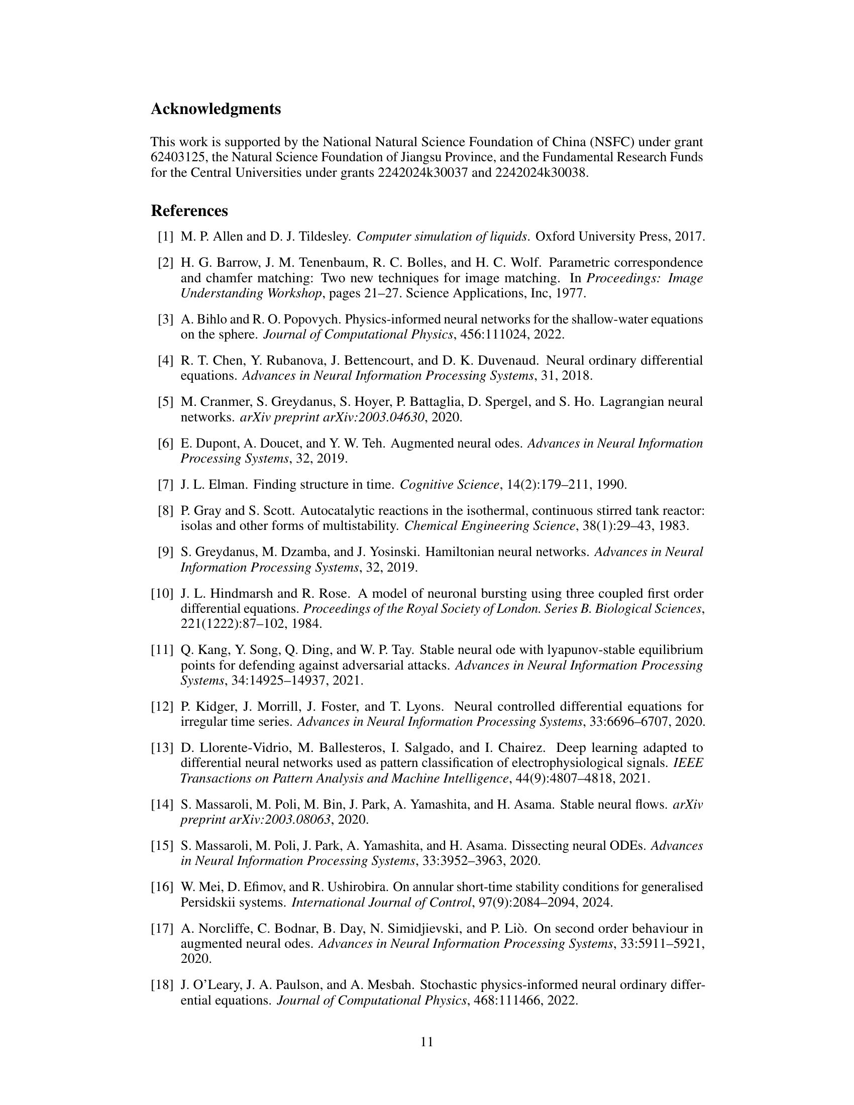
This figure presents a performance comparison of CSODE models with varying numbers of sub-networks. A heatmap shows the validation loss for different combinations of network width and number of subnetworks. A scatter plot displays the relationship between training and validation losses during training for models with 1 to 5 subnetworks, at a fixed network width of 512. Models with lower losses (closer to the bottom-left corner) perform better. The scatter plot also illustrates the balance between training and validation performance.
This figure compares the prediction results of CSODE and NODE models against the ground truth trajectory at three different training epochs (400, 600, and 800). It visually demonstrates CSODE’s superior performance in accurately learning and extrapolating the trajectory, even beyond the observed data points, showcasing its better understanding of underlying dynamics.

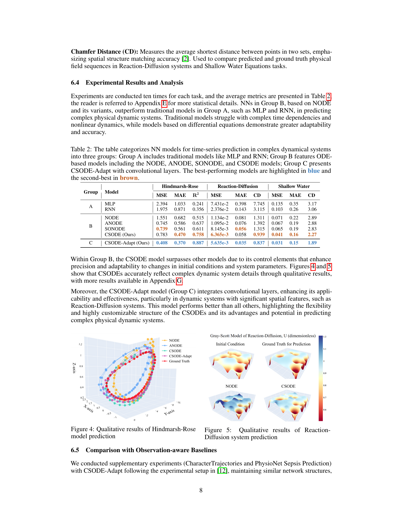
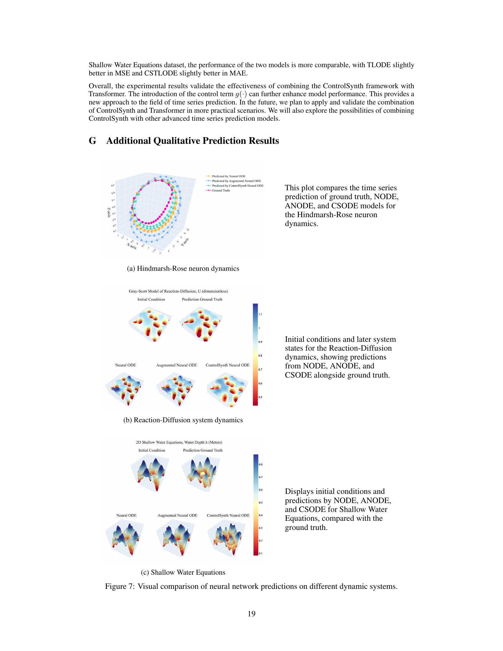
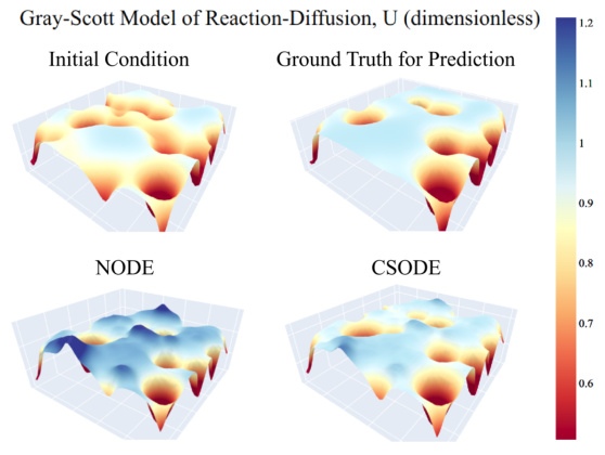
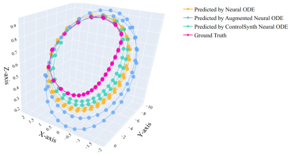
This figure presents a qualitative comparison of the predictions generated by three different neural ordinary differential equation (NODE) models: NODE, Augmented NODE (ANODE), and ControlSynth NODE (CSODE), against the ground truth for three distinct dynamic systems. These systems are the Hindmarsh-Rose neuron model, a Reaction-Diffusion system, and the Shallow Water Equations. The figure shows 3D plots visualizing the initial conditions, ground truth dynamics, and predictions from each model. This allows for a visual assessment of the accuracy and ability of each model to capture complex and nonlinear dynamical behaviors. Note that the CSODE demonstrates improved ability to capture the detail of the underlying dynamics.
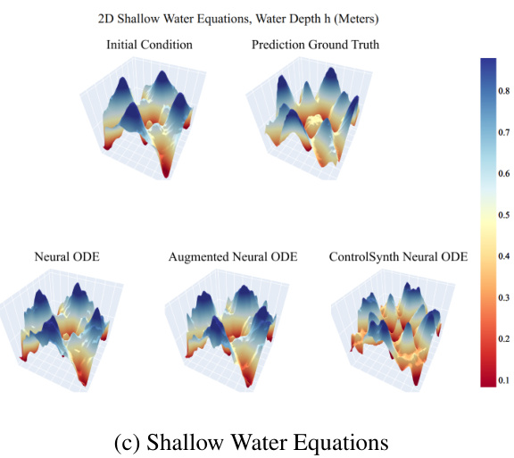
This figure presents a qualitative comparison of the predictions made by three different neural ordinary differential equation (NODE) models: NODE, ANODE, and CSODE. Each model’s performance is shown alongside the ground truth for three different dynamical systems: the Hindmarsh-Rose neuron model (a), the Reaction-Diffusion system (b), and the Shallow Water Equations (c). The visualization helps illustrate how each model approximates the complex dynamics of these systems, highlighting CSODE’s improved accuracy and ability to learn the time-dependent structures in the data.
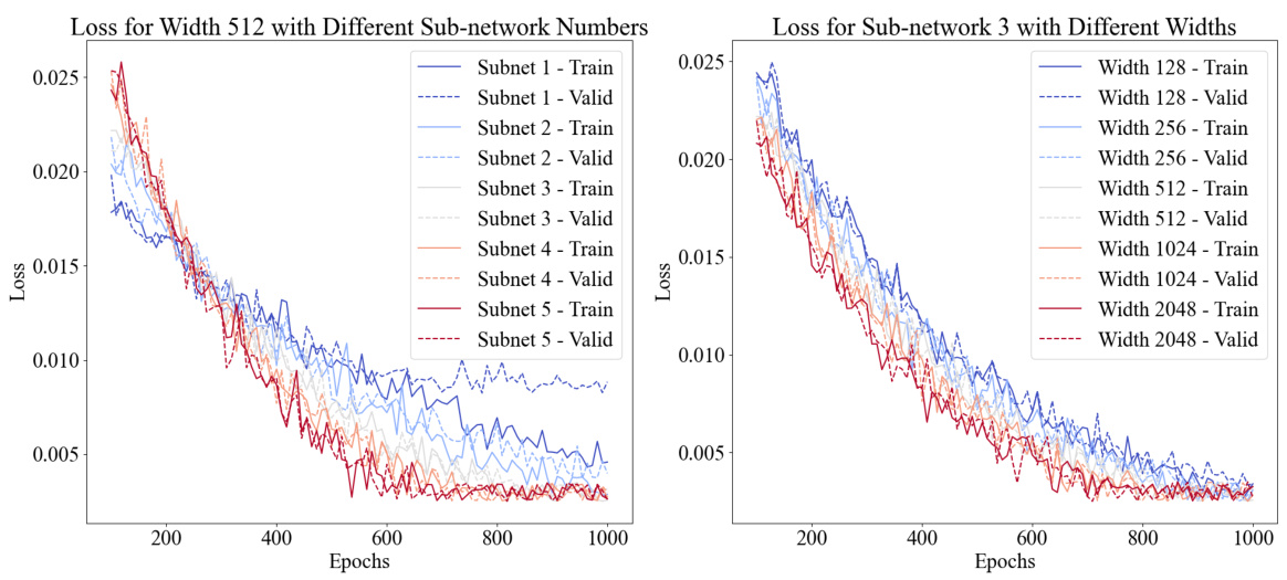
This figure shows two plots visualizing the training and validation loss curves for CSODEs under different configurations. The left plot shows the results of varying the number of sub-networks while keeping the network width fixed at 512. The right plot, on the other hand, varies the network width while keeping the number of sub-networks constant at 3. Each plot demonstrates how changes in these architectural parameters affect the model’s convergence and overall performance during training. The plots illustrate the impact of different network configurations on the model’s training and validation losses, providing insights into the trade-offs between model complexity and performance.
More on tables

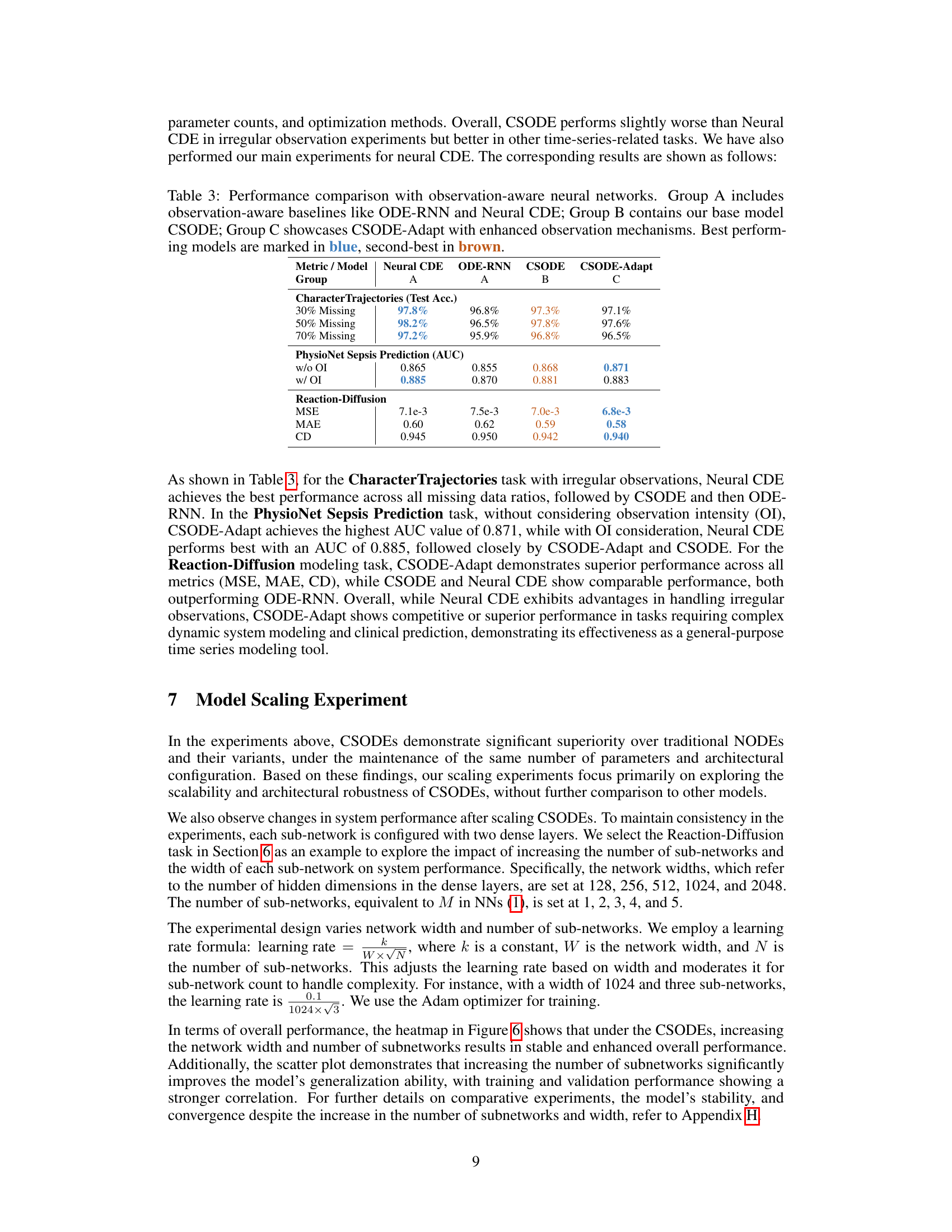
This table compares the performance of various neural network models (traditional MLP and RNN, ODE-based NODE, ANODE, SONODE, and CSODE, and CSODE-Adapt) on three complex time series prediction tasks (Hindmarsh-Rose neuron dynamics, Reaction-Diffusion system, and Shallow Water Equations). The models are grouped into categories based on their architecture and the best-performing models in each task are highlighted.
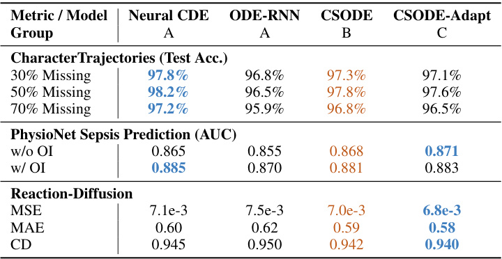
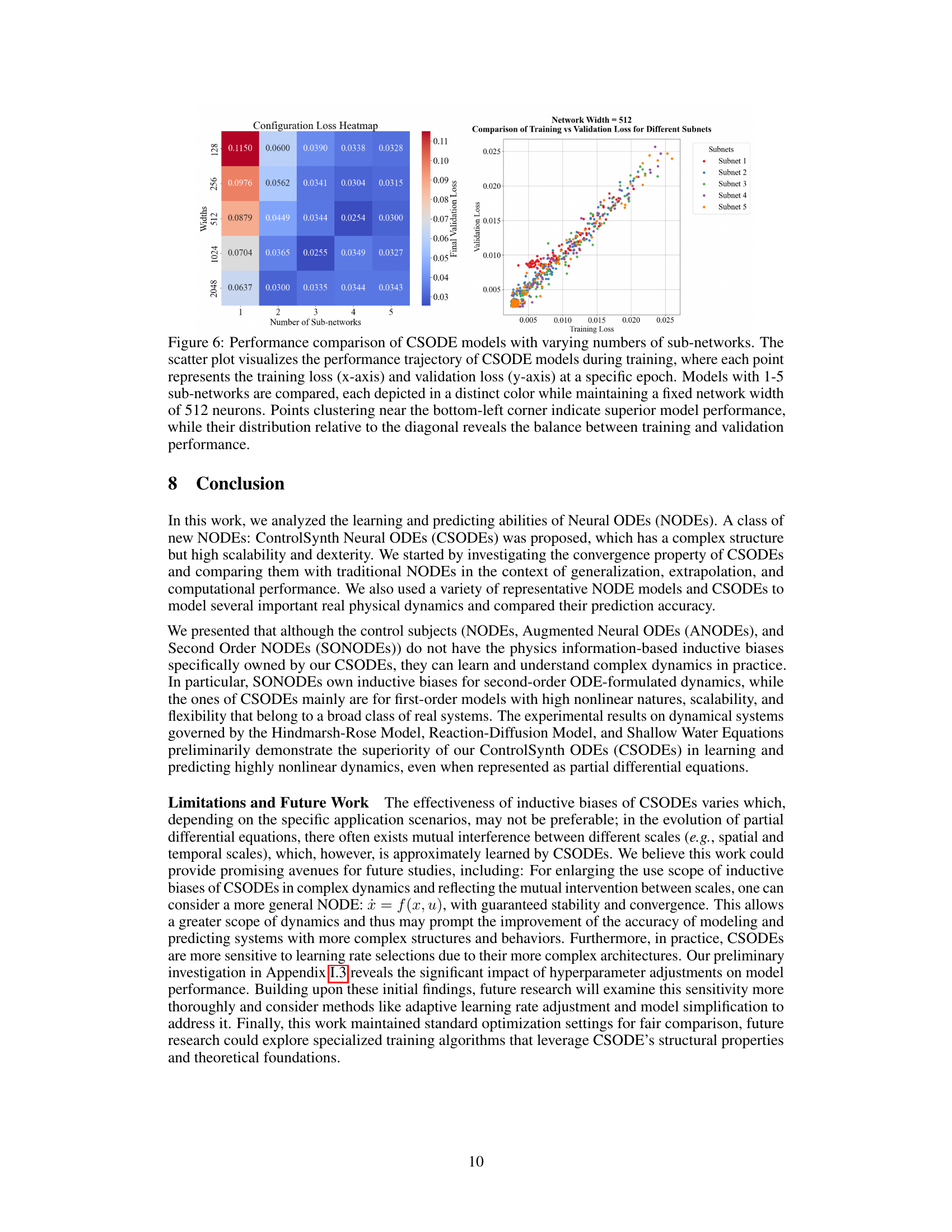
This table compares the performance of CSODE and its variant (CSODE-Adapt) against other observation-aware neural network models (Neural CDE, ODE-RNN) across three different tasks: Character Trajectories prediction with varying levels of missing data, PhysioNet Sepsis Prediction with and without observation intensity, and Reaction-Diffusion system modeling. The metrics used to evaluate performance vary depending on the task, and include test accuracy, AUC, MSE, MAE, and Chamfer Distance. The best performing model in each category is highlighted in blue, and the second-best in brown. The table shows that CSODE and its variant perform competitively with state-of-the-art methods, sometimes even surpassing them in specific tasks.

This table presents a comparison of the performance of several neural ordinary differential equation (NODE) based models on the MNIST image classification dataset. The models compared include NODE, Augmented Neural ODE (ANODE), Second Order Neural ODE (SONODE), and ControlSynth Neural ODE (CSODE). The metrics used for comparison are test error rate, number of parameters, floating-point operations per second (FLOPS), average batch processing time, and peak memory usage. The results show that CSODE achieves a slightly better test error rate (0.39%) compared to other models, with comparable performance in terms of computational efficiency and memory usage.

This table compares the performance of various Neural Ordinary Differential Equation (NODE) based models on the MNIST image classification task. Metrics include test error rate, number of parameters, floating-point operations per second (FLOPS), average batch processing time, and peak memory usage. The models compared are NODE, Augmented Neural ODE (ANODE), Second Order Neural ODE (SONODE), and ControlSynth Neural ODE (CSODE). The table shows that CSODE achieves a slightly lower test error rate than the other models while maintaining comparable computational efficiency.
This table compares the performance of various neural ordinary differential equation (NODE) based models on the MNIST image classification task. The models compared include NODE, Augmented Neural ODE (ANODE), Second Order Neural ODE (SONODE), and ControlSynth Neural ODE (CSODE). For each model, the table reports the test error rate (%), the number of parameters (#Params), floating-point operations per second (FLOPS), average batch processing time (Time in seconds), and peak memory usage (MB). This allows for a direct comparison of the computational efficiency and resource requirements of each model.

This table compares the performance of various neural network models (traditional MLP and RNN, ODE-based NODE, ANODE, SONODE, and CSODE, and CSODE-Adapt) on three complex dynamical systems: Hindmarsh-Rose neuron, Reaction-Diffusion, and Shallow Water Equation. The models are grouped by their architectural approach, and their performance is evaluated using MSE, MAE, R2 (for Hindmarsh-Rose only), and CD (for Reaction-Diffusion and Shallow Water only). The best and second-best performing models in each group and task are highlighted.

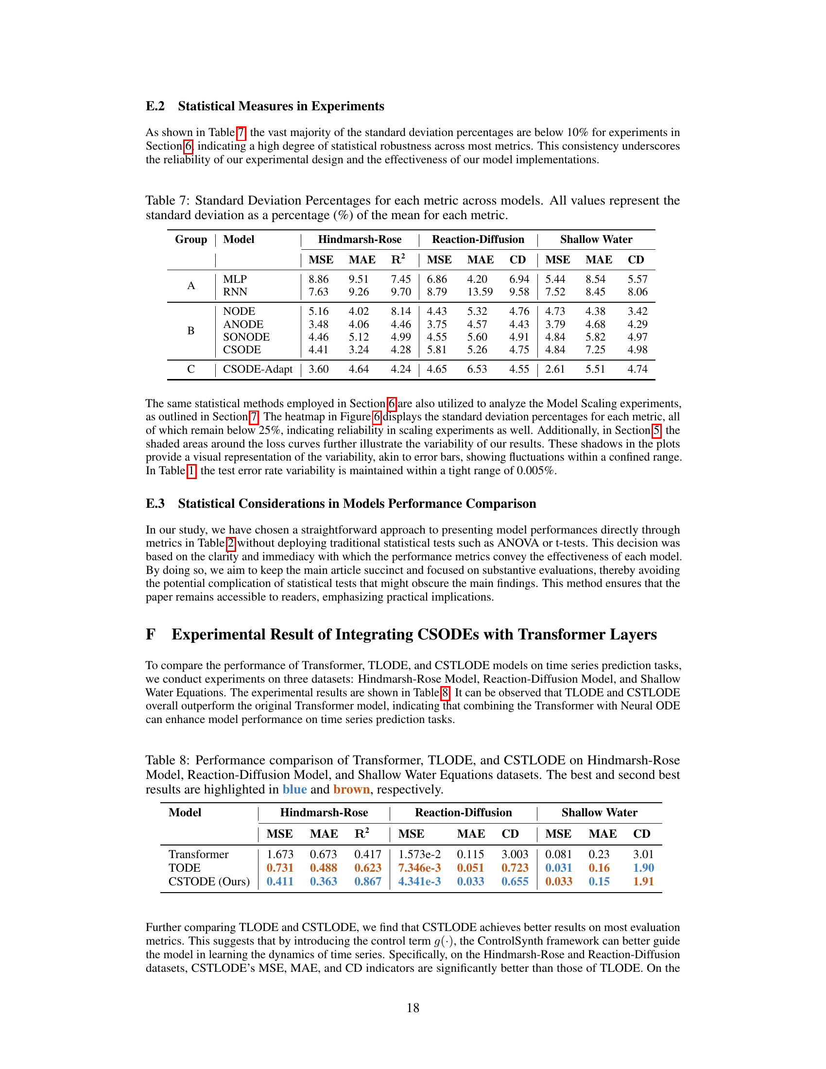
This table compares the performance of three different models (Transformer, TLODE, and CSTODE) on three different datasets (Hindmarsh-Rose, Reaction-Diffusion, and Shallow Water Equations). The performance is measured using MSE, MAE, R2 (for Hindmarsh-Rose only), and CD. The best performing model for each metric and dataset is highlighted in blue, with the second-best highlighted in brown. This table illustrates the relative effectiveness of integrating Neural ODEs with Transformer layers, and the benefit of adding a control term (as in CSTODE).
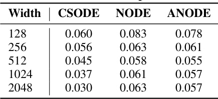
This table presents a comparison of the Mean Absolute Error (MAE) achieved by three different neural ordinary differential equation (NODE) models – CSODE, NODE, and ANODE – across various network widths (128, 256, 512, 1024, and 2048) when applied to the Reaction-Diffusion task. Lower MAE values indicate better model performance. The table helps illustrate how the models’ accuracy changes with varying network capacity.
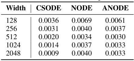
This table presents a comparison of the Mean Squared Error (MSE) achieved by three different neural ordinary differential equation (NODE) models: ControlSynth Neural ODEs (CSODEs), standard NODEs, and Augmented NODEs (ANODEs). The comparison is made across varying network widths (128, 256, 512, 1024, and 2048) in the context of the Reaction-Diffusion task. Lower MSE values indicate better model performance. The table shows that CSODE consistently outperforms the other two models across all widths, demonstrating its superior performance and efficiency in this task.

This table compares the Mean Absolute Error (MAE) achieved by using two different numerical solvers, Euler and Dopri5, for three different Neural Ordinary Differential Equation (NODE) models: NODE, ANODE, and CSODE. The comparison highlights the impact of solver choice on the accuracy of these models in solving the Reaction-Diffusion problem. Lower MAE values indicate better performance.

This table compares the performance of four different neural ordinary differential equation (NODE) models on the MNIST image classification task. The models compared are NODE, ANODE, SONODE, and CSODE. The metrics used for comparison include test error rate, the number of parameters, floating-point operations per second (FLOPS), average batch processing time, and peak memory usage. The table shows that CSODE achieves a slightly lower test error rate than the other models, while maintaining comparable computational performance in terms of FLOPS, time, and memory usage.

This table presents a performance comparison of four different neural ordinary differential equation (NODE) based models on the MNIST image classification task. The models compared are NODE, ANODE, SONODE, and CSODE. The metrics used for comparison are test error rate, number of parameters, floating-point operations per second (FLOPS), average batch processing time, and peak memory usage. The results demonstrate that although CSODEs theoretically involves iterative computation of g(u), it does not significantly reduce computational efficiency in practice.
Full paper#
