TL;DR#
Many physical systems are modeled by PDEs where both the continuous fields and discrete parameters are unknown. Traditional methods solve these problems separately, leading to inconsistencies. This often involves computationally expensive simulations. Furthermore, assessing uncertainty propagation through these separate processes is difficult.
This paper introduces FUSE, a unified framework that jointly predicts continuous quantities and infers discrete parameter distributions. This significantly improves accuracy and robustness by amortizing computational cost through a pre-training step. The framework is demonstrated on two complex test cases: full-body haemodynamics and atmospheric large-eddy simulation, showing superior performance compared to existing methods. The key is to unify forward and inverse problems within a single framework, thus improving both prediction and inference.
Key Takeaways#
Why does it matter?#
This paper is important because it presents FUSE, a novel and flexible framework for solving the joint prediction of continuous fields and statistical estimation of underlying discrete parameters in PDEs. This addresses a critical challenge in various scientific domains by significantly improving accuracy and robustness through a unified approach, impacting research in areas like climate science, fluid dynamics, and biomechanics.
Visual Insights#

🔼 This figure illustrates the FUSE framework, which is a unified forward-inverse model for parametric PDEs. It shows how finite-dimensional parameters (ξ) are used to predict both continuous functions (u) and (s) using a combination of neural operators and flow-matching posterior estimation. The figure highlights the flow of information through the model: From finite-dimensional inputs to infinite-dimensional outputs and back again, with the use of band-limited Fourier transforms to bridge the gap between the finite and infinite dimensional spaces.
read the caption
Figure 1: FUSE models a posterior distribution over finite-dimensional parameters ξ given infinite-dimensional functions u with du components (channels). It learns other continuous functions s with ds channels from parameters ξ. Band-limited Fourier transforms and a lifting operator act as a bridge between finite and infinite dimensions for the forward problem. Likewise, as inference models such as FMPE or NPE require fixed-size inputs, the operator layers are conjoined with a band-limited Fourier transform to learn a fixed-size representation of the input function.
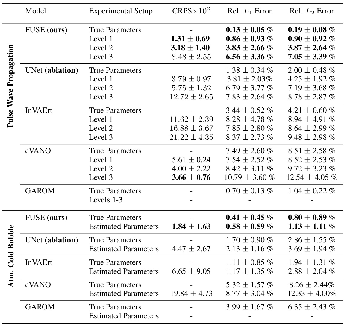
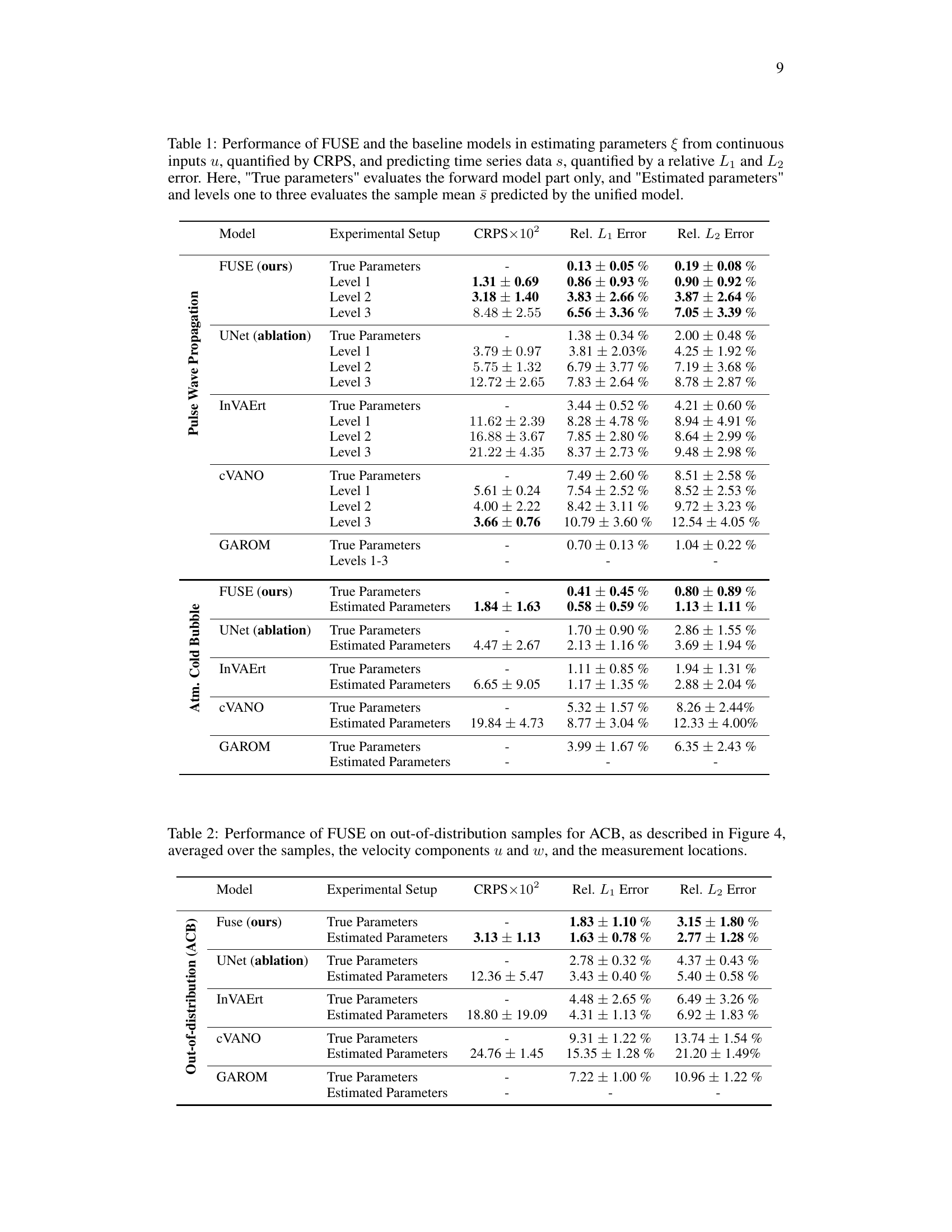
🔼 This table presents a comparison of the performance of the proposed FUSE model against several baseline models in two tasks: estimating parameters (ξ) from continuous inputs (u) and predicting time series data (s). The performance is measured using three metrics: CRPS (Continuous Ranked Probability Score) for parameter estimation and relative L₁ and L₂ errors for time series prediction. The table includes results for three different levels of input information for pulse wave propagation. For the atmospheric cold bubble, both true parameter and estimated parameter results are presented.
read the caption
Table 1: Performance of FUSE and the baseline models in estimating parameters ξ from continuous inputs u, quantified by CRPS, and predicting time series data s, quantified by a relative L₁ and L2 error. Here, 'True parameters' evaluates the forward model part only, and 'Estimated parameters' and levels one to three evaluates the sample mean Predicted by the unified model.
In-depth insights#
Unified Forward-Inverse#
A unified forward-inverse approach in PDE modeling is a powerful strategy, combining the prediction of continuous fields (forward) with the estimation of underlying parameters (inverse). This joint approach promises significant gains in accuracy and robustness compared to tackling these problems separately. By amortizing the computational cost through a joint pre-training step, the method offers an efficient solution for various applications. The key lies in building a flexible framework that consistently estimates both continuous quantities and the distributions of discrete parameters. The success relies on the synergy between forward and inverse models, with propagated uncertainty playing a critical role. This unified approach is particularly effective when dealing with incomplete or noisy data, as it can effectively handle uncertainty propagation. Therefore, it has the potential to be highly beneficial for various domains requiring both prediction and parameter estimation from limited information.
FNO and FMPE#
The research paper section on “FNO and FMPE” likely details the integration of two powerful deep learning architectures to solve a unified forward-inverse problem for parametric PDEs. FNO (Fourier Neural Operator) excels at learning mappings between function spaces, making it ideal for handling the continuous nature of PDE solutions. FMPE (Flow-Matching Posterior Estimation), on the other hand, is a powerful technique for efficiently estimating the probability distribution of parameters, addressing the inverse problem. The combination is innovative because it leverages FNO’s ability to create accurate surrogates and FMPE’s strength in uncertainty quantification. By jointly training these models, the method aims to achieve significantly improved accuracy and robustness in both the forward prediction and parameter inference tasks. The authors likely present a novel mathematical framework, a unified objective function for joint training, and possibly showcase the approach’s effectiveness through experiments involving complex PDE systems.
ACB and PWP tests#
The ACB (Atmospheric Cold Bubble) and PWP (Pulse Wave Propagation) tests in this research paper serve as crucial validation experiments. They showcase the model’s ability to handle complex, realistic physical systems governed by PDEs. ACB tests, modeling a turbulent atmospheric phenomenon, assess the model’s predictive accuracy for highly nonlinear dynamics involving sharp velocity gradients. Meanwhile, PWP tests, simulating blood flow in the human arterial network, demonstrate its capability for accurate parameter inference and uncertainty quantification in a complex biological system. The choice of these two distinct test cases highlights the model’s versatility and robustness, extending beyond simple, idealized scenarios to real-world applications. The results from these experiments, quantified using appropriate metrics, offer convincing evidence of the model’s effectiveness in both forward surrogate modeling and inverse parameter estimation tasks. The comparisons to various baseline models further strengthen the claims of improved performance and robustness. The thoughtful inclusion of ACB and PWP tests significantly enhances the credibility and impact of the research findings.
Uncertainty Propagation#
The concept of uncertainty propagation is central to the paper’s methodology. The authors highlight the importance of understanding how uncertainties in input parameters (e.g., those characterizing the system conditions or model parameters) affect the accuracy of predictions from the forward model. They argue that tackling this issue through joint pre-training of inverse and forward models provides a more robust and accurate approach than conventional methods, which typically address these two problems separately. By integrating both problems within the same framework, inconsistencies are reduced, and the accuracy and reliability of both inverse estimation and surrogate predictions are improved. The paper demonstrates this improvement empirically with results on pulse wave propagation and atmospheric cold bubble simulations. The method, by its design, quantifies the uncertainty in predictions by propagating input uncertainty through the models to obtain an ensemble of predictions. This is important for evaluating the reliability of a model’s outputs in contexts where exact values of input parameters are unknown.
Future Work#
The authors suggest several promising avenues for future research. Extending FUSE to handle scenarios with measurement errors and non-physical parameters is crucial for real-world applications. The current framework assumes perfect measurements, a limitation that needs addressing. Incorporating uncertainty from measurement errors into the model would enhance robustness. Also, exploring parameterizations where parameters are functions (e.g., space-time dependent) would be relevant. This extension would require a more sophisticated representation of the latent space, potentially using neural operators or other function-valued representations, to account for these complexities. Investigating different forward and inverse models within the FUSE framework would improve its performance and flexibility. The FNO and FMPE used are just examples, and others might be more suitable for specific problems. Finally, extending FUSE to higher-dimensional spaces (e.g., 3D) and more complex PDEs is a necessary step toward broader applicability. Scaling the model to larger datasets and more computationally intensive problems will require efficient implementation and potentially algorithmic modifications.
More visual insights#
More on figures

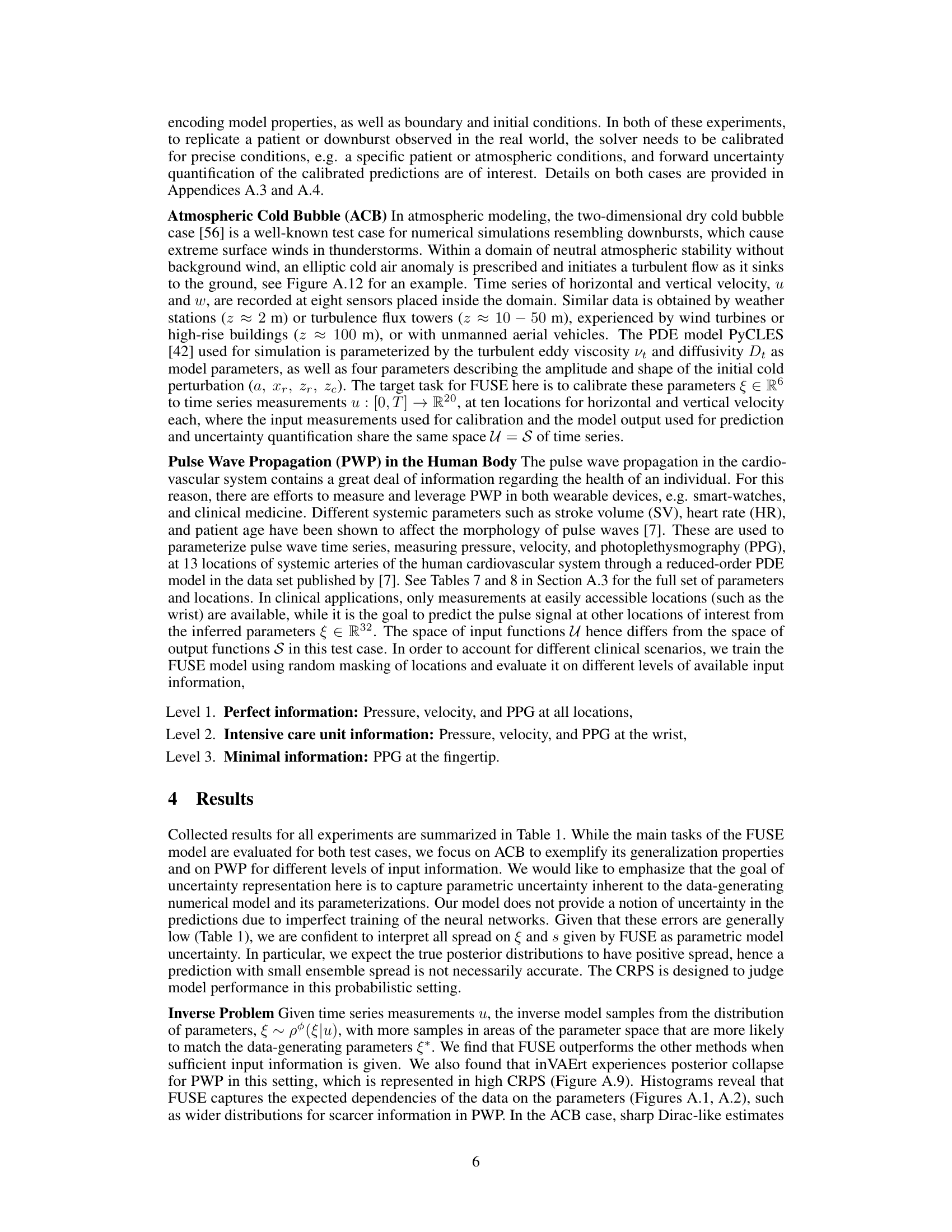
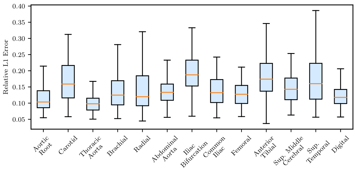
🔼 This figure shows box plots visualizing the relative L1 errors in time series predictions for the Atmospheric Cold Bubble (ACB) experiment. Two scenarios are presented: (a) the forward problem, where the prediction is based on the true parameters, and (b) the unified prediction, where the ensemble mean prediction is based on the input time series data. The plots illustrate the accuracy of the model’s predictions at different measurement locations and how the uncertainty propagates in the forward and unified tasks. Each box plot represents the error distribution at a specific location, with the box indicating the interquartile range (IQR), the line inside representing the median, and the whiskers extending to the minimum and maximum values.
read the caption
Figure A.21: ACB, propagated uncertainty: Box plots of relative errors in the time series predictions at each location.

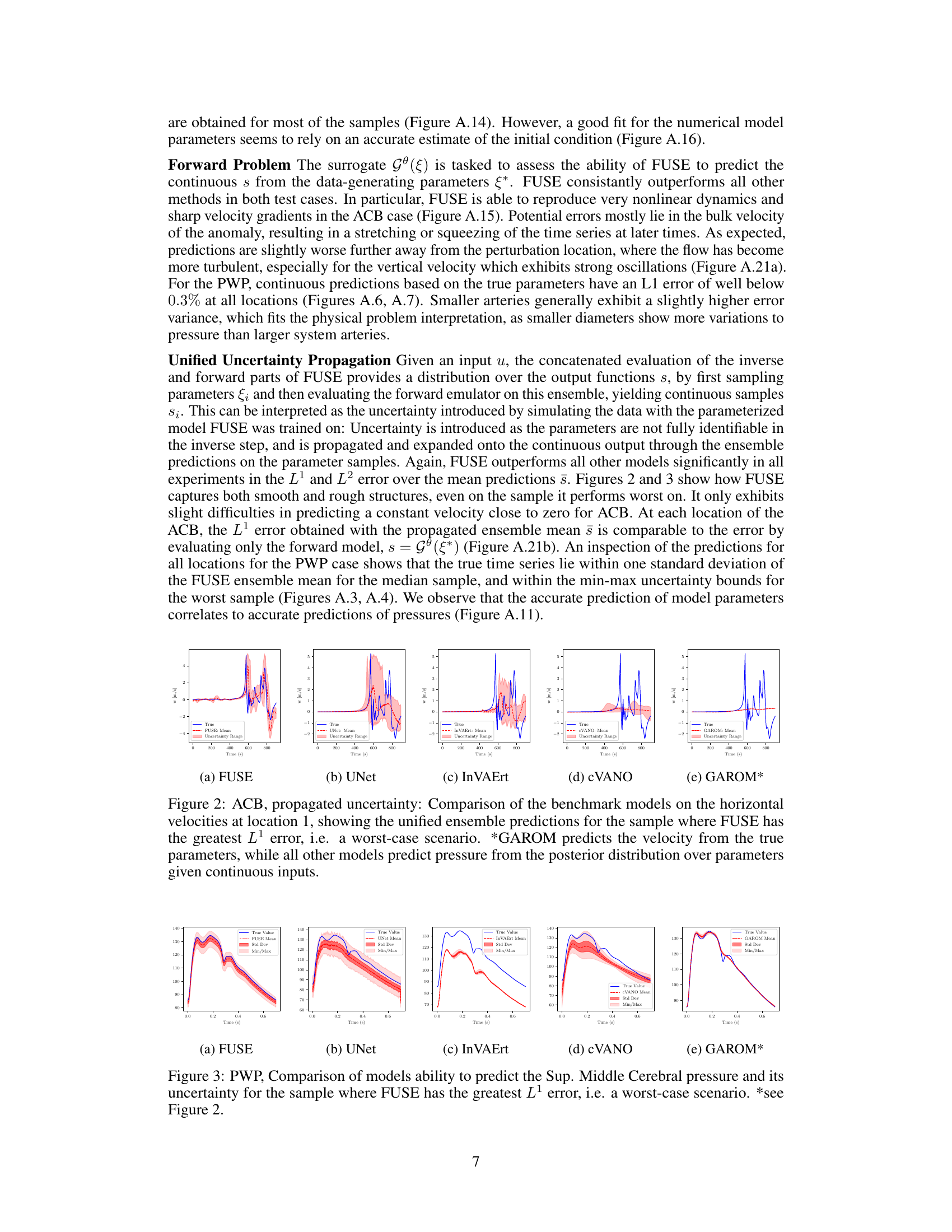
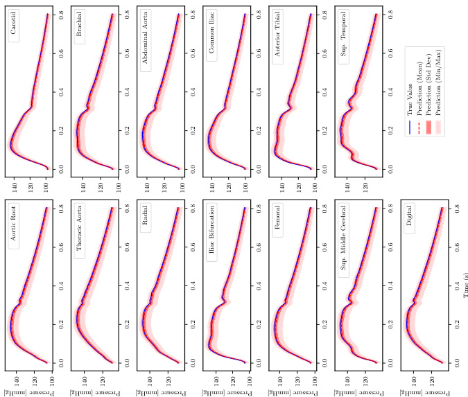
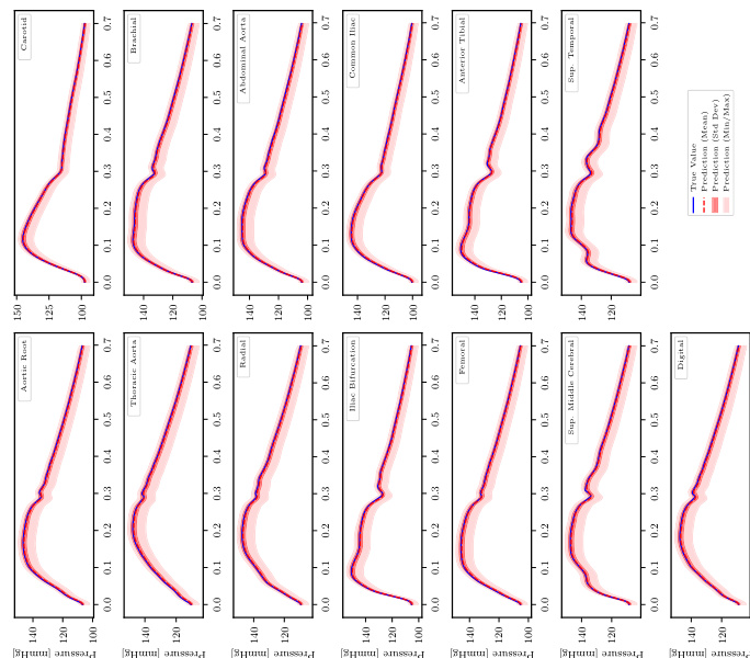
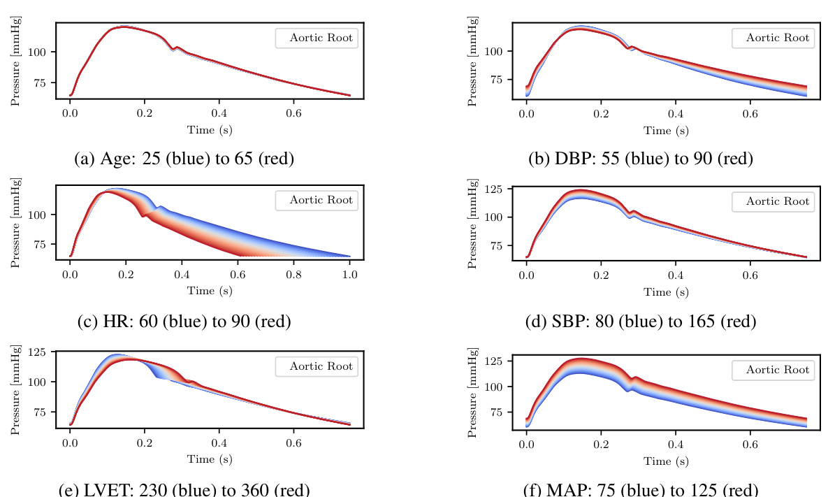
🔼 This figure shows the pressure time series at different locations in the human arterial network. The blue line represents the true value, while the red line represents the mean prediction from the FUSE model. The shaded area shows the standard deviation (Std Dev) and minimum/maximum values (Min/Max) of the predictions based on the ensemble generated by FUSE. The different subplots represent different levels of available information, showing how the accuracy of the predictions varies depending on the amount of available data. In general, as more information is available, the predictions become more accurate.
read the caption
Figure A.3: PWP, propagated uncertainty: Pressure time series for the sample with the median rel. L₁ Error for each level of available input information.

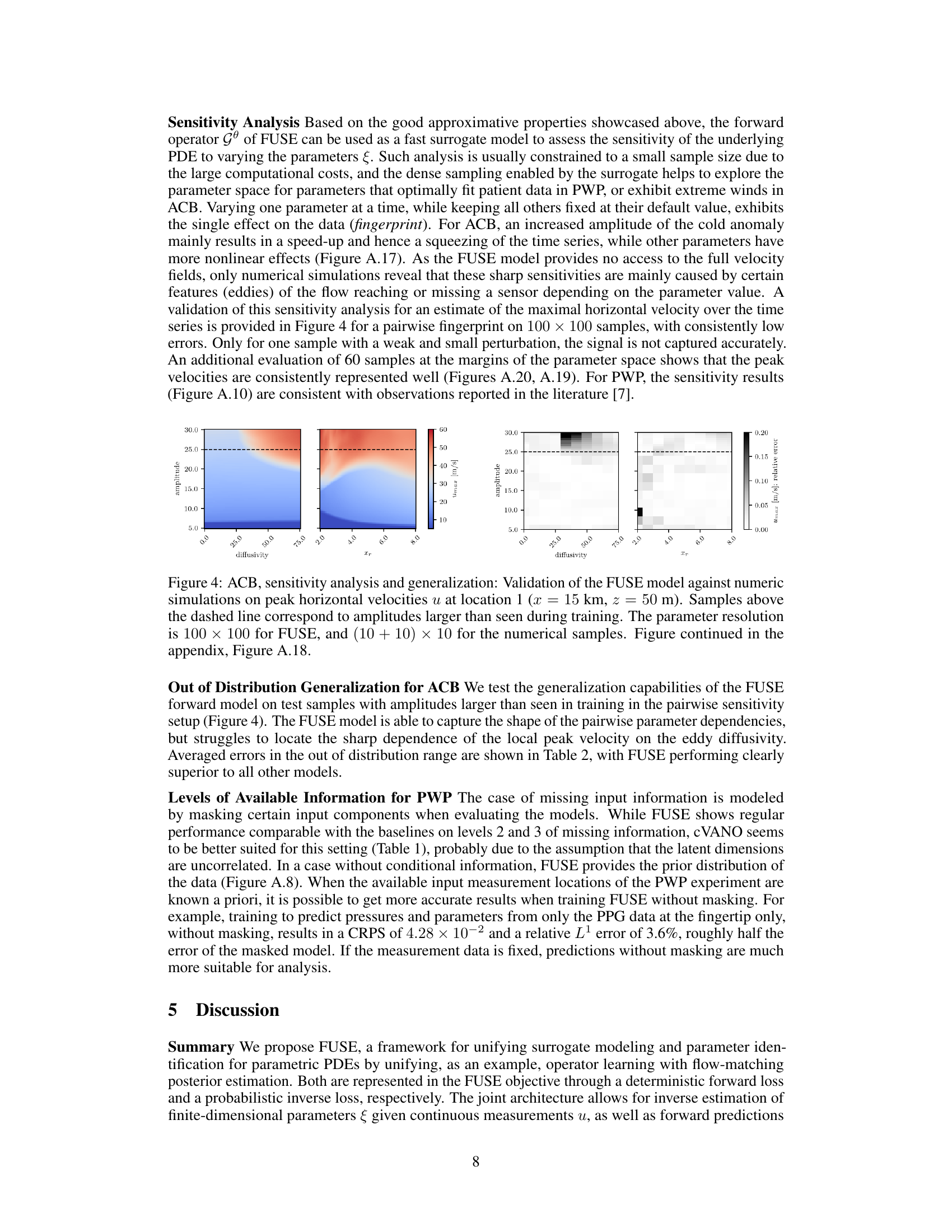
🔼 This figure presents a sensitivity analysis for the Atmospheric Cold Bubble (ACB) experiment, comparing the performance of the FUSE model against numerical simulations. The analysis focuses on peak horizontal velocities at two different locations: one further away from the perturbation center (left) and one closer (right). The figure displays four key metrics in a 2x2 arrangement for each location. Top row shows relative error and difference between FUSE and the numerical simulations. Bottom row shows the maximum velocity calculated by the numerical model and the maximum velocity from FUSE. This comparison helps evaluate how well FUSE captures the sensitivity of the ACB model to changes in its parameters.
read the caption
Figure A.18: ACB, sensitivity analysis, continuation of Fig. 4: Validation of the FUSE model against numeric simulations on peak horizontal velocities u at location 1 (left, further away from the perturbation center) and 5 (right, closer). From top to bottom: relative error between FUSE and the numerical model, difference between FUSE and the numerical model, maximum velocity calculated by the numerical model, maximum velocity calculated by FUSE.
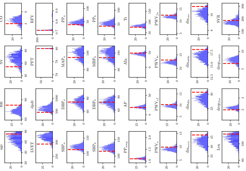
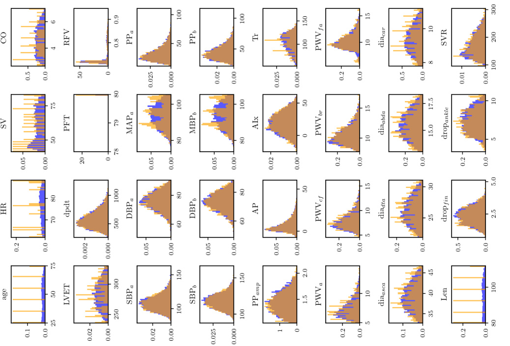
🔼 This figure shows the distribution of inferred parameters from the inverse problem for pulse wave propagation (PWP) for three different levels of input information. Each level represents a different amount of available data, ranging from ‘perfect information’ (all locations) to ‘minimal information’ (only the fingertip). Histograms are shown for each parameter, illustrating how the accuracy and precision of the parameter estimates change based on the amount of available input data. The median Continuous Ranked Probability Score (CRPS) is used to select the sample shown for each level. Lower CRPS values indicate better agreement with the true parameter values.
read the caption
Figure A.1: PWP, inverse problem: Histograms for the sample with the median CRPS for each level of available input information.
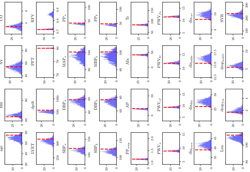
🔼 This figure shows the probability density functions (histograms) of the estimated parameters for three different levels of available input information in pulse wave propagation (PWP). The distributions represent the uncertainty in estimating parameters from the given measurements. The median CRPS (Continuous Ranked Probability Score) indicates the overall goodness of fit. The histograms allow us to visualize the distribution and spread of the estimated parameters for each level of information, revealing how much uncertainty is introduced.
read the caption
Figure A.1: PWP, inverse problem: Histograms for the sample with the median CRPS for each level of available input information.
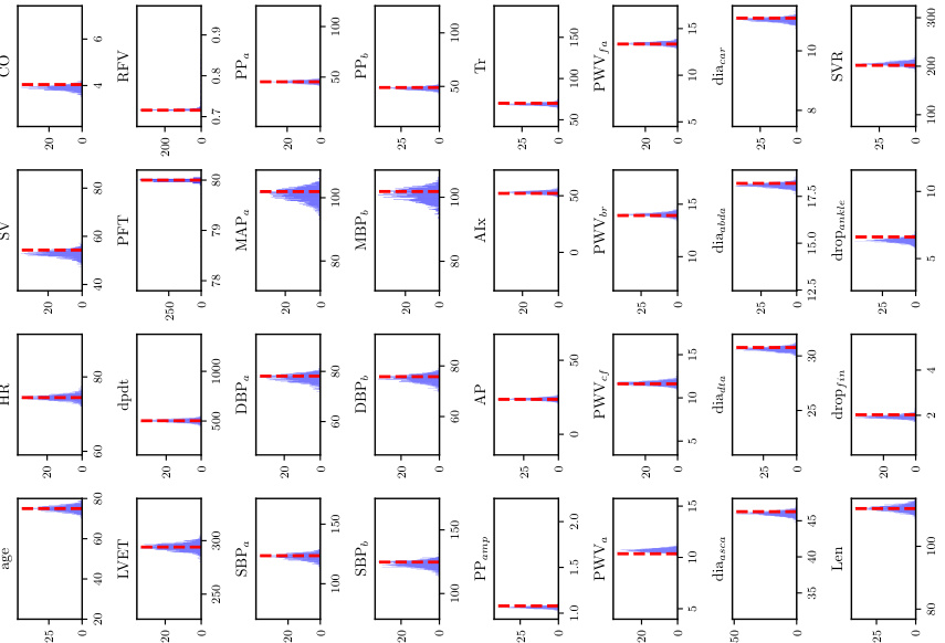
🔼 The figure shows the probability distributions obtained by the inverse model for the parameters of the pulse wave propagation problem for three different levels of input information. The distributions are shown in histograms, with each bin representing a range of parameter values. The x-axis represents the parameter values, while the y-axis represents the frequency of occurrence of each parameter value in the sample. The figure is useful to visualize how the uncertainty in the parameter estimates changes based on the amount of input information available.
read the caption
Figure A.1: PWP, inverse problem: Histograms for the sample with the median CRPS for each level of available input information.
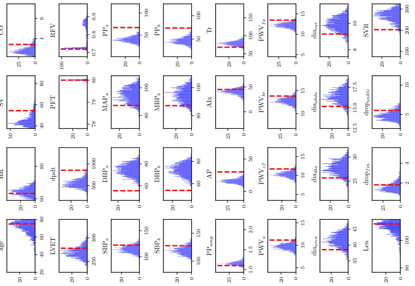
🔼 This figure displays histograms of the posterior distribution of parameters, inferred by the inverse model for each level of available information for a sample with median CRPS. The histograms show the distribution over the parameters given by the inverse FUSE model. For each level, distributions are shown for all parameters. The vertical dashed lines represent the true parameter values from the data-generating process. The histograms show that FUSE captures the expected dependencies of the data on the parameters. In particular, for the case of scarcer information, FUSE produces wider distributions over the parameters.
read the caption
Figure A.1: PWP, inverse problem: Histograms for the sample with the median CRPS for each level of available input information.
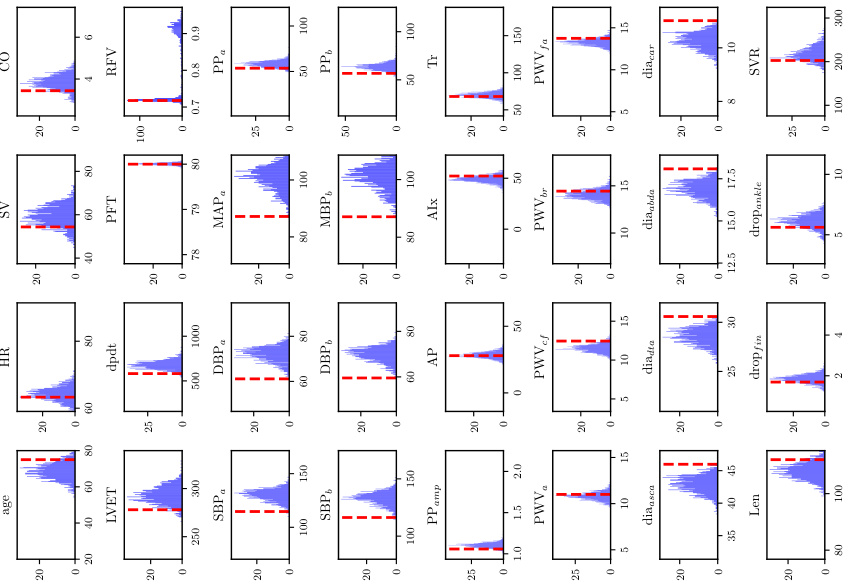
🔼 This figure displays histograms of the parameter samples obtained from the inverse problem (parameter inference) of the FUSE model for the Pulse Wave Propagation (PWP) experiment. It shows the results for three different levels of input information (information levels 1, 2, and 3), indicating the amount of data available for the inference task. For each level, the histograms represent the probability distribution of the inferred parameters, illustrating how the availability of input information affects the accuracy of parameter estimation. The median Continuous Ranked Probability Score (CRPS) value is selected for display.
read the caption
Figure A.1: PWP, inverse problem: Histograms for the sample with the median CRPS for each level of available input information.
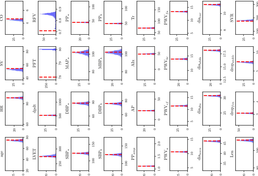
🔼 This figure shows the distributions of the inferred parameters for the pulse wave propagation (PWP) problem using the FUSE model. The histograms represent the probability distributions of the parameters obtained from the inverse problem for three different levels of input information (Level 1, Level 2, Level 3). Each level corresponds to a different amount of available physiological data. The median Continuous Ranked Probability Score (CRPS) is shown for each level, indicating the overall quality of the parameter estimation by the FUSE model given different input information levels. The red dashed vertical lines represent the true values of the parameters from the data generating simulation.
read the caption
Figure A.1: PWP, inverse problem: Histograms for the sample with the median CRPS for each level of available input information.

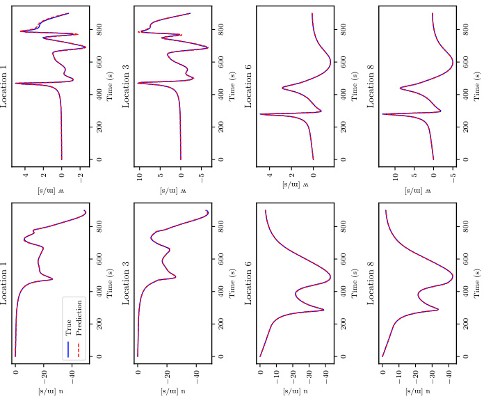
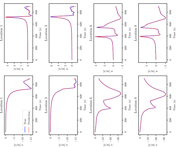
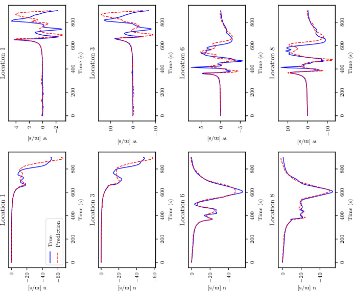
🔼 This figure shows the pressure time series at different locations in the human arterial network for the sample with the median relative L1 error. Three information levels are presented: perfect information, intensive care unit information, and minimal information. The true values are shown in black, the mean prediction in blue, standard deviation in light blue, and min/max range in pink. This visualization helps understand the uncertainty propagation from input to output, demonstrating how data scarcity affects the accuracy and uncertainty of the prediction.
read the caption
Figure A.3: PWP, propagated uncertainty: Pressure time series for the sample with the median rel. L₁ Error for each level of available input information.
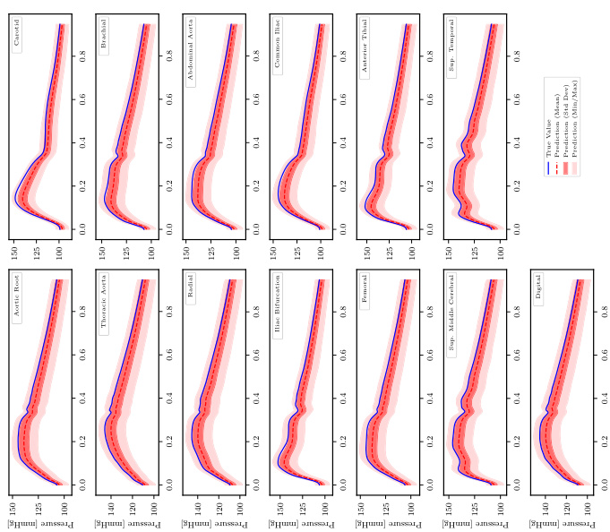
🔼 This figure shows the pressure time series for the sample with median relative L1 error at different levels of input information. Each subplot represents a different artery location in the human arterial network. The blue line shows the true pressure, the solid red line shows the mean of the pressure predictions, the dashed red lines represent the standard deviation of the prediction, and the dotted red lines represent the min/max range of the prediction. The figure demonstrates the ability of FUSE to predict pressure and the uncertainty associated with the predictions under different conditions. The uncertainty is higher when less information is available, as expected.
read the caption
Figure A.3: PWP, propagated uncertainty: Pressure time series for the sample with the median rel. L¹ Error for each level of available input information.
🔼 This figure visualizes the pressure time series at various locations in the arterial network for three different levels of input information (information levels 1, 2, and 3). For each location, the true pressure values are shown in blue, along with the mean predicted pressure in red, the standard deviation in light red, and the minimum and maximum pressure in a light red shaded area. This shows how the accuracy of pressure prediction changes with different levels of input data availability, highlighting the impact of incomplete information on the model’s accuracy.
read the caption
Figure A.3: PWP, propagated uncertainty: Pressure time series for the sample with the median rel. L₁ Error for each level of available input information.
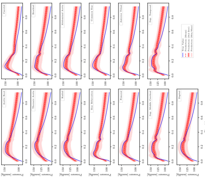
🔼 This figure shows the pressure time series at different locations in the human arterial network for three different levels of available information (information level 1, 2, and 3). The true pressure values are shown in blue. The predictions of the FUSE model, which accounts for the uncertainty in the model parameters, are shown in red. The mean prediction is represented by the solid red line, the standard deviation by the shaded area, and the minimum and maximum values by the dashed red lines. The figure demonstrates that the accuracy of the FUSE model predictions increases with increasing information level.
read the caption
Figure A.3: PWP, propagated uncertainty: Pressure time series for the sample with the median rel. L¹ Error for each level of available input information.

🔼 The figure shows pressure time series for three different levels of available input information. The true values and the predictions from the model are shown for each location. The predictions include the mean, standard deviation, and minimum/maximum values. This visualization helps to understand the uncertainty associated with each level of input information in predicting pressure time series.
read the caption
Figure A.3: PWP, propagated uncertainty: Pressure time series for the sample with the median rel. L¹ Error for each level of available input information.
🔼 This figure displays the pressure time series at various locations in the human arterial network for the sample exhibiting median relative L1 error across three levels of input information (perfect, intensive care unit, and minimal). It presents the true pressure values along with the mean, standard deviation, and minimum/maximum of the predictions obtained from the FUSE model. The aim is to showcase the model’s accuracy in predicting pressure while highlighting uncertainty propagation from incomplete information levels.
read the caption
Figure A.3: PWP, propagated uncertainty: Pressure time series for the sample with the median rel. L¹ Error for each level of available input information.
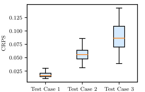
🔼 This figure shows the performance of the forward and inverse components of the FUSE model under different levels of input information (Test Cases 1-3). The box plots illustrate the CRPS for the inverse problem (parameter estimation) and the L1 error for the forward and unified problems (prediction of the continuous function s). As expected, accuracy decreases as less input information is available.
read the caption
Figure A.5: PWP: Box plots of the errors of the forward and inverse components of FUSE, as reported in Table 1, for different levels of available input information ('test cases'). For the inverse problem, parameter samples ξᵢ are sampled from pº(ξ|u). For the forward problem, the output function s is predicted based on the true parameter values ξ* ~ ρ(ξ|u). For the unified problem evaluating both the inverse and forward model parts, the means of the ensemble prediction sᵢ from inferred parameters ξᵢ ~ pº(ξ|u) is compared to the true output time series s. As information is removed from the input in the different cases, it becomes more difficult to estimate s.
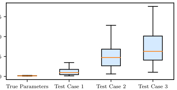
🔼 This figure shows box plots comparing the performance of the FUSE model’s forward and inverse components, along with a unified approach, across three levels of input information. The results highlight the trade-off between accuracy and the availability of input data.
read the caption
Figure A.5: PWP: Box plots of the errors of the forward and inverse components of FUSE, as reported in Table 1, for different levels of available input information ('test cases'). For the inverse problem, parameter samples ξi are sampled from pº(ξ|u). For the forward problem, the output function s is predicted based on the true parameter values ξ* ~ ρ(ξ|u). For the unified problem evaluating both the inverse and forward model parts, the means of the ensemble prediction si from inferred parameters ξi ~ pº(ξ|u) is compared to the true output time series s. As information is removed from the input in the different cases, it becomes more difficult to estimate s.
🔼 This figure presents the results of the pulse wave propagation (PWP) experiment, comparing the true pressure time series with the predictions from FUSE at different levels of input information. The median L1 error was used to select the sample shown. The plots display pressure at different locations in the arterial system (Aortic Root, Carotid, etc.) across three levels of input information (1, 2, and 3). It visualizes the accuracy of FUSE’s predictions (mean, standard deviation, min/max range) compared to the true values, demonstrating FUSE’s performance on both smooth and rough structures, particularly its handling of uncertainty propagation.
read the caption
Figure A.3: PWP, propagated uncertainty: Pressure time series for the sample with the median rel. L¹ Error for each level of available input information.

🔼 This figure shows the pressure time series at different locations in the arterial network for the sample with median relative L1 error for three different levels of input information (perfect information, intensive care unit information, and minimal information). Each subfigure shows the true pressure (black line), the predicted mean pressure from FUSE (red line), the standard deviation (light red shading), and the minimum/maximum predictions (light red lines).
read the caption
Figure A.3: PWP, propagated uncertainty: Pressure time series for the sample with the median rel. L₁ Error for each level of available input information.
🔼 This figure shows the probability distributions of the parameters inferred by the FUSE model for the pulse wave propagation (PWP) experiment. The histograms represent the posterior distributions pº(ξ|u) for different levels of input information (information levels 1, 2, and 3). Each level represents a decreasing amount of input data used to infer the parameters. The median CRPS (Continuous Ranked Probability Score) sample is shown for each level. The CRPS measures how well the predicted distribution matches a single true value.
read the caption
Figure A.1: PWP, inverse problem: Histograms for the sample with the median CRPS for each level of available input information.

🔼 The figure shows the distributions of the estimated parameters from the inverse model of FUSE for the sample with the median CRPS, across three different levels of available input information. Each level represents a decreasing amount of data, illustrating how the uncertainty in the parameter estimates increases as less data is available. The histograms visualize the probability density of each parameter at each level, showing the spread and uncertainty in the estimations. This provides insights into the robustness and reliability of FUSE across varying data conditions.
read the caption
Figure A.1: PWP, inverse problem: Histograms for the sample with the median CRPS for each level of available input information.
🔼 This figure visualizes the pressure time series at different locations in the human arterial network for three levels of input information: perfect, ICU, and minimal. The median sample (in terms of relative L1 error) is shown, illustrating pressure with error bars indicating standard deviation and min/max range. This demonstrates how uncertainty in input data propagates through the model to impact the precision of pressure predictions at different artery locations.
read the caption
Figure A.3: PWP, propagated uncertainty: Pressure time series for the sample with the median rel. L¹ Error for each level of available input information.
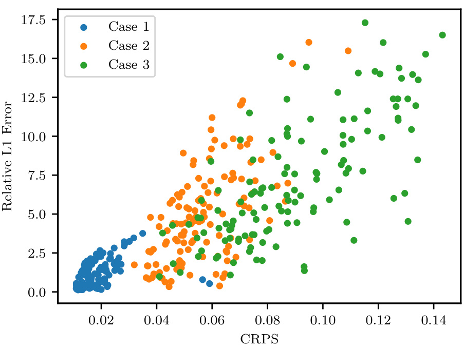
🔼 This figure shows the correlation between the continuous relative L1 error and the discrete CRPS error for the pulse wave propagation (PWP) experiment. The three different cases represent varying levels of available input information. The x-axis represents the CRPS error, indicating the accuracy of the model’s parameter estimation. The y-axis represents the relative L1 error, indicating the accuracy of the model’s predictions. The plot helps visualize how uncertainty in parameter estimation (higher CRPS) relates to the uncertainty in prediction (higher L1 error). Different colors represent different levels of input data, allowing analysis of the impact of data availability on model accuracy.
read the caption
Figure A.11: PWP: Correlation of the errors between continuous (L¹) and discrete (CRPS) parameters for different levels of available input information ('cases').
🔼 This figure illustrates the FUSE (Fast Unified Simulation and Estimation for PDEs) framework. It shows how the model handles both finite-dimensional parameters (ξ) and infinite-dimensional functions (u and s). The finite-dimensional parameters are used to predict the continuous functions, and the model learns the relationship between them. The use of band-limited Fourier transforms is highlighted to enable the model to work with both finite and infinite dimensional data. This framework jointly predicts continuous quantities and infers distributions of discrete parameters which is a central concept in the paper.
read the caption
Figure 1: FUSE models a posterior distribution over finite-dimensional parameters ξ given infinite-dimensional functions u with du components (channels). It learns other continuous functions s with ds channels from parameters ξ. Band-limited Fourier transforms and a lifting operator act as a bridge between finite and infinite dimensions for the forward problem. Likewise, as inference models such as FMPE or NPE require fixed-size inputs, the operator layers are conjoined with a band-limited Fourier transform to learn a fixed-size representation of the input function.

🔼 This figure illustrates the architecture of the FUSE (Fast Unified Simulation and Estimation for PDEs) framework. It shows how the framework integrates finite-dimensional parameters (ξ) with infinite-dimensional functions (u and s) using a combination of operator layers (e.g., Fourier Neural Operators) and a band-limited Fourier transform. The model is designed to learn a joint mapping between parameters and both continuous outputs and latent space, enabling both surrogate prediction and parameter inference within a single framework.
read the caption
Figure 1: FUSE models a posterior distribution over finite-dimensional parameters ξ given infinite-dimensional functions u with du components (channels). It learns other continuous functions s with ds channels from parameters ξ. Band-limited Fourier transforms and a lifting operator act as a bridge between finite and infinite dimensions for the forward problem. Likewise, as inference models such as FMPE or NPE require fixed-size inputs, the operator layers are conjoined with a band-limited Fourier transform to learn a fixed-size representation of the input function.
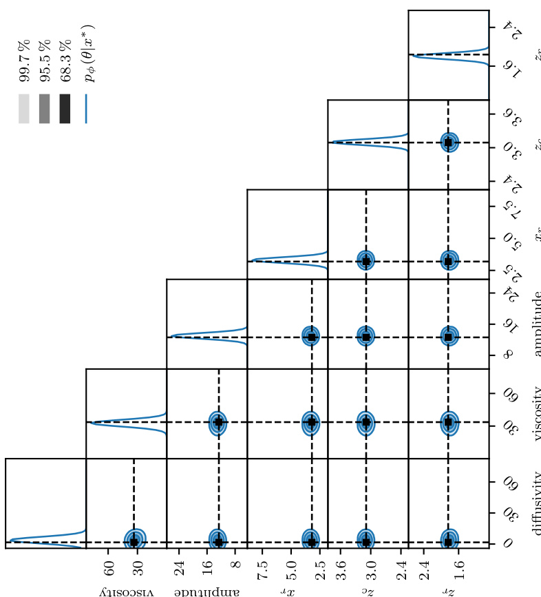
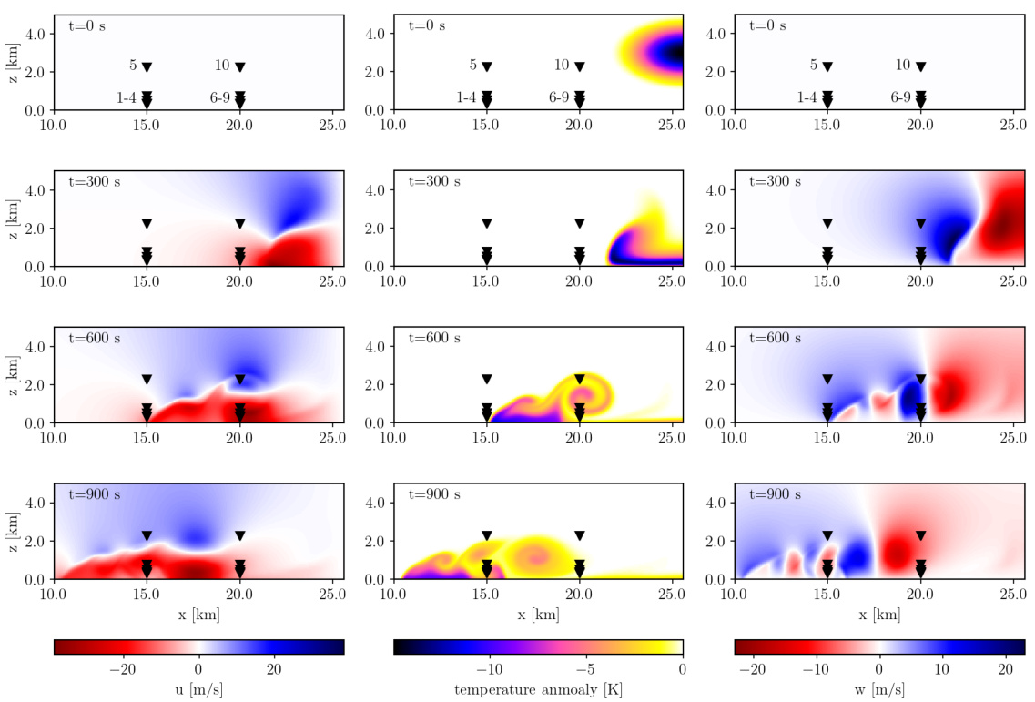
🔼 This figure shows the results of the inverse problem for the Atmospheric Cold Bubble (ACB) experiment. For each parameter, histograms display the probability density of the sampled parameters using the FUSE model, given the continuous measurements. The true parameter values are shown as dashed vertical lines for comparison, allowing for a visual assessment of how well FUSE is able to recover the true parameter distributions based on the measurements. The shaded regions show the 68.3%, 95.5%, and 99.7% confidence intervals of the distributions.
read the caption
Figure A.14: ACB, inverse problem: Samples drawn from the parameter distributions given continuous time series data. The true parameter values are marked with dashed lines, while the predicted distributions are given in blue shading.
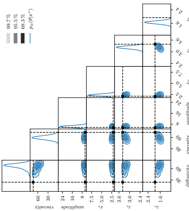
🔼 This figure shows the results of the inverse problem for the Atmospheric Cold Bubble (ACB) case study. The histograms represent the posterior distributions of the model parameters (amplitude, viscosity, diffusivity, horizontal radius (Xr), vertical location (Zc), vertical radius (Zr)) given continuous time series measurements. The true parameter values are shown as dashed lines for comparison. The blue shading represents the predicted probability densities. The plot is split into two subfigures: (a) shows the worst-performing sample from the test set and (b) shows the median-performing sample. This visualization allows for assessing how well the model recovers the underlying parameter values from noisy observations.
read the caption
Figure A.14: ACB, inverse problem: Samples drawn from the parameter distributions given continuous time series data. The true parameter values are marked with dashed lines, while the predicted distributions are given in blue shading.
🔼 This figure shows the pressure time series at different locations in the human arterial network for three different levels of input information (information levels 1, 2, and 3). The true values are shown in black, the mean prediction by the FUSE model is in red, the standard deviation is shown in pink, and the min/max range is depicted in light red. The plot shows how well the FUSE model predicts the pressure at various locations with varying amounts of available input data. Lower information levels mean less input data is used for the prediction, which would result in higher uncertainty (larger pink regions) and less accurate predictions (larger difference between red and black curves).
read the caption
Figure A.3: PWP, propagated uncertainty: Pressure time series for the sample with the median rel. L¹ Error for each level of available input information.
🔼 This figure shows the pressure time series at different locations in the arterial network for the sample with the median relative L1 error. The three subfigures represent different levels of available input information: (a) perfect information, (b) ICU information, and (c) minimal information. For each level, the true pressure (black line) is compared to the prediction mean (blue line) and the prediction uncertainty (red shaded area). The uncertainty is given by the standard deviation of ensemble predictions.
read the caption
Figure A.3: PWP, propagated uncertainty: Pressure time series for the sample with the median rel. L¹ Error for each level of available input information.
🔼 This figure shows the distribution of parameters inferred by the inverse model for three different levels of available input information (information levels 1, 2, and 3). Each level represents a decreasing amount of information available to the model. Histograms illustrate the probability distribution of each parameter given the input data for the sample that yielded a median CRPS (continuous ranked probability score) across all samples at each information level. The closer the distributions are to the true parameter values (represented by vertical dashed lines), the better the model’s ability to infer the parameters.
read the caption
Figure A.1: PWP, inverse problem: Histograms for the sample with the median CRPS for each level of available input information.

🔼 This figure displays histograms visualizing the posterior distributions of the parameters inferred by the FUSE model for the pulse wave propagation (PWP) experiments. Each sub-figure corresponds to one level of available input information (information levels 1-3), representing different amounts of data. The histograms show the probability density of each parameter given the measured data for the sample with the median CRPS value. By showing how these distributions differ across different levels of information, the figure illustrates the model’s ability to learn and incorporate the uncertainty in the inputs and the subsequent impact on parameter estimation. The vertical red lines represent the true parameter values used to generate the data.
read the caption
Figure A.1: PWP, inverse problem: Histograms for the sample with the median CRPS for each level of available input information.

🔼 This figure displays the histograms of the parameters inferred from continuous time-series measurements of pulse wave propagation (PWP) in the human arterial network. Histograms are shown for the sample with the median Continuous Ranked Probability Score (CRPS), for each of the three levels of available input information (perfect information, intensive care unit information, and minimal information). The true values of the parameters are indicated by the red dashed lines.
read the caption
Figure A.1: PWP, inverse problem: Histograms for the sample with the median CRPS for each level of available input information.
🔼 This figure visualizes the pressure time series at different locations in the human arterial network for three different levels of input information. The median rel. L¹ error sample is selected to be shown. The plot displays the true values (black), the predicted means (blue), the standard deviations (light blue), and the min/max values (red). It illustrates the accuracy and uncertainty of the FUSE model’s predictions compared to the actual pressure measurements across various arterial locations and levels of data availability.
read the caption
Figure A.3: PWP, propagated uncertainty: Pressure time series for the sample with the median rel. L¹ Error for each level of available input information.
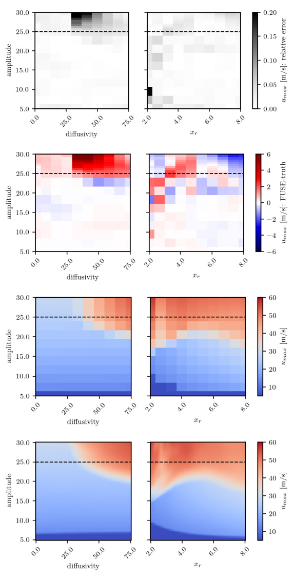
🔼 This figure shows a comparison of the FUSE model’s performance against numerical simulations in predicting peak horizontal velocities at two different locations in an atmospheric cold bubble (ACB) scenario. The comparison is based on the relative error, the difference, and the maximum velocities calculated by both methods. The results demonstrate the FUSE model’s ability to accurately capture the dynamics of the ACB.
read the caption
Figure A.18: ACB, sensitivity analysis, continuation of Fig. 4: Validation of the FUSE model against numeric simulations on peak horizontal velocities u at location 1 (left, further away from the perturbation center) and 5 (right, closer). From top to bottom: relative error between FUSE and the numerical model, difference between FUSE and the numerical model, maximum velocity calculated by the numerical model, maximum velocity calculated by FUSE.
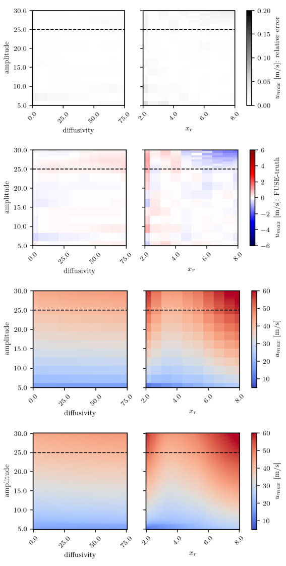
🔼 This figure shows the results of a sensitivity analysis for the Atmospheric Cold Bubble (ACB) experiment. It compares the predictions of the FUSE model against numerical simulations for peak horizontal velocities at two different locations. The top row displays the relative error between the FUSE model and the numerical simulation. The second row shows the absolute difference between the two. The third and fourth rows present the maximum velocity calculated by the numerical model and the FUSE model, respectively. The results demonstrate the accuracy and reliability of the FUSE model in predicting the dynamic behavior of the ACB system.
read the caption
Figure A.18: ACB, sensitivity analysis, continuation of Fig. 4: Validation of the FUSE model against numeric simulations on peak horizontal velocities u at location 1 (left, further away from the perturbation center) and 5 (right, closer). From top to bottom: relative error between FUSE and the numerical model, difference between FUSE and the numerical model, maximum velocity calculated by the numerical model, maximum velocity calculated by FUSE.
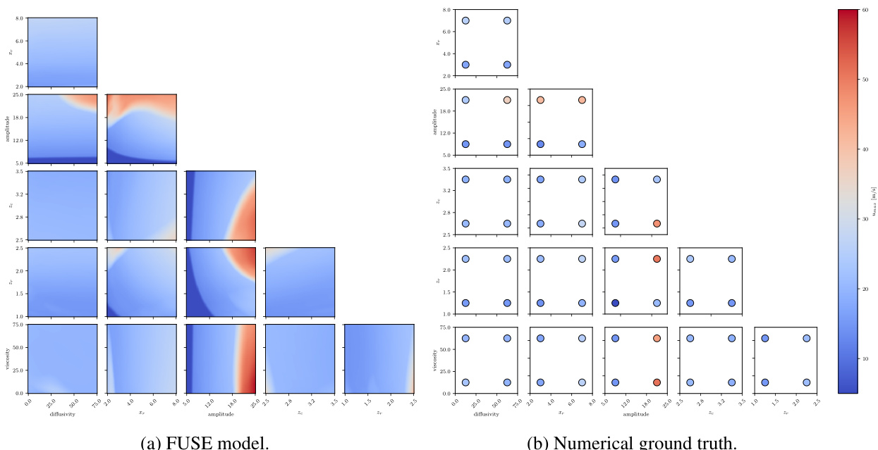
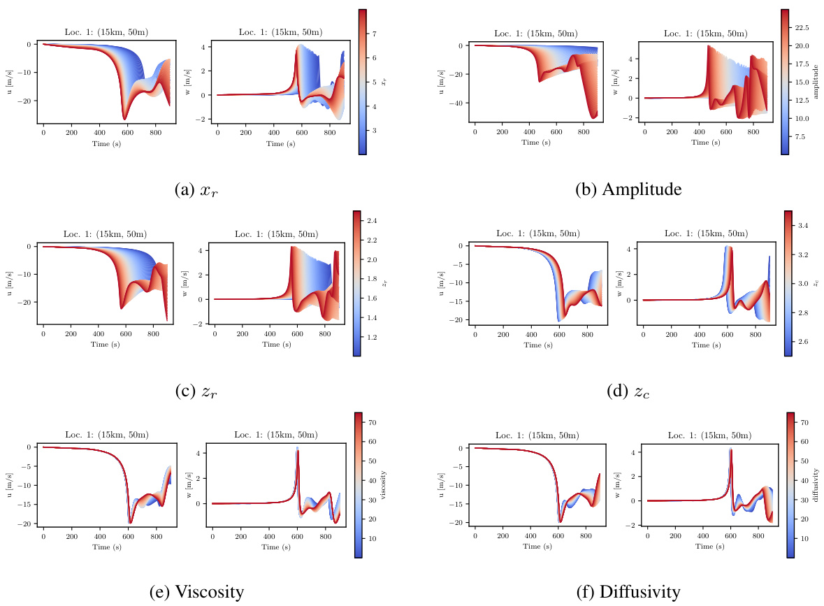
🔼 This figure shows the sensitivity analysis of the Atmospheric Cold Bubble (ACB) model. It displays the peak horizontal velocities at a specific location (15 km, 50 m) for different combinations of model parameters. Two plots are shown: one for the FUSE model and one for the numerical ground truth. Each plot illustrates how peak velocities vary with changes in the model’s parameters.
read the caption
Figure A.19: ACB, sensitivity analysis: Peak horizontal velocities u at location 1 (x = 15 km, z = 50 m), sampled for pairwise combinations of the parameters, while keeping all others at their default value. For the neural model (a), 100 samples are drawn for each parameter, corresponding to 150,000 evaluations. For the numerical model (b), four simulations were run per pair of parameters, with each taking values corresponding to 1/6 and 5/6 of the parameter range, corresponding to 60 model evaluations.
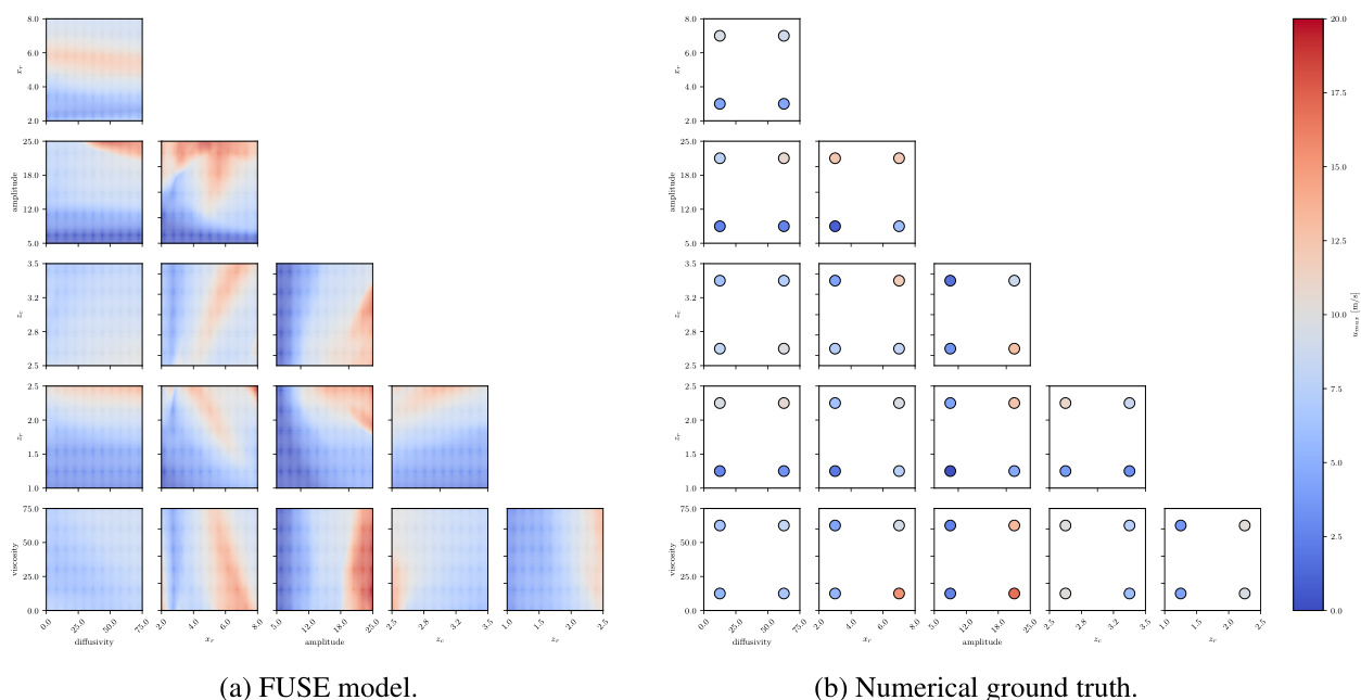
🔼 This figure shows the sensitivity analysis of the ACB model. The left panel shows the results from the FUSE model, while the right panel shows the results from the numerical ground truth. The top row shows the pairwise combinations of parameters. The bottom row shows the peak horizontal velocities for each pairwise combination of parameters.
read the caption
Figure A.19: ACB, sensitivity analysis: Peak horizontal velocities u at location 1 (x = 15 km, z = 50 m), sampled for pairwise combinations of the parameters, while keeping all others at their default value. For the neural model (a), 100 samples are drawn for each parameter, corresponding to 150,000 evaluations. For the numerical model (b), four simulations were run per pair of parameters, with each taking values corresponding to 1/6 and 5/6 of the parameter range, corresponding to 60 model evaluations.
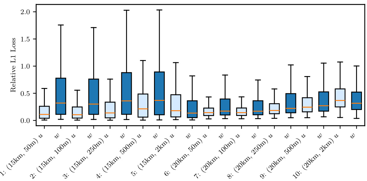
🔼 This figure shows box plots of the relative L1 errors in the time series predictions for both the forward and unified problems in the ACB experiment. The forward problem uses the true parameters to generate the predictions, while the unified problem uses the inferred parameters from the input time series. The x-axis represents the eight measurement locations, and the y-axis represents the relative L1 error. The box plots show the median, interquartile range (IQR), and whiskers extending to 1.5 times the IQR. The purpose is to visualize and compare the accuracy of the model’s predictions in different conditions.
read the caption
Figure A.21: ACB, propagated uncertainty: Box plots of relative errors in the time series predictions at each location.
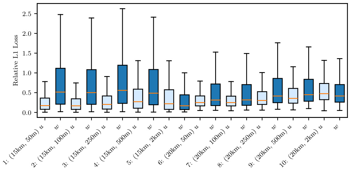
🔼 This figure shows box plots illustrating the relative L1 errors in the time series predictions for the Atmospheric Cold Bubble (ACB) experiment. The errors are broken down by location, showing the difference between the predictions and the true values. The plots are separated into two subfigures: (a) shows the errors when using the true parameters for the forward problem and (b) shows the errors from a unified prediction (both inverse and forward models). The x-axis displays the various measurement locations. The y-axis represents the relative L1 error values. The box plots themselves show the median, first and third quartiles, and the range of the data. Whiskers extend to the maximum and minimum values within 1.5 times the interquartile range.
read the caption
Figure A.21: ACB, propagated uncertainty: Box plots of relative errors in the time series predictions at each location.
More on tables
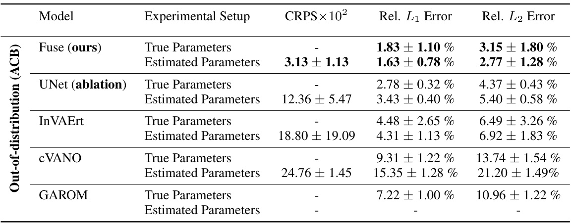
🔼 This table presents a comparison of the performance of the proposed FUSE model against several baseline models in two tasks: estimating parameters (ξ) from continuous inputs (u) and predicting time series data (s). The performance is measured using the Continuous Ranked Probability Score (CRPS) for parameter estimation and relative L₁ and L₂ errors for time series prediction. The table includes results for three different levels of input information, reflecting varying amounts of available data. The ‘True parameters’ row shows the performance of the forward model only, using the true parameters, while ‘Estimated parameters’ shows the performance when using parameters estimated by the models.
read the caption
Table 1: Performance of FUSE and the baseline models in estimating parameters ξ from continuous inputs u, quantified by CRPS, and predicting time series data s, quantified by a relative L₁ and L₂ error. Here, 'True parameters' evaluates the forward model part only, and 'Estimated parameters' and levels one to three evaluates the sample mean š predicted by the unified model.

🔼 This table summarizes the performance comparison between the proposed FUSE model and several baseline models on two different tasks: parameter estimation and time series prediction. The performance is evaluated using CRPS for parameter estimation and relative L1 and L2 errors for time series prediction. The table also shows performance at different levels of input information.
read the caption
Table 1: Performance of FUSE and the baseline models in estimating parameters ξ from continuous inputs u, quantified by CRPS, and predicting time series data s, quantified by a relative L₁ and L₂ error. Here, 'True parameters' evaluates the forward model part only, and 'Estimated parameters' and levels one to three evaluates the sample mean Predicted by the unified model.
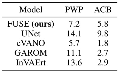
🔼 This table shows the number of millions of parameters used in each model for the Pulse Wave Propagation (PWP) and Atmospheric Cold Bubble (ACB) experiments. It allows for a comparison of model complexity between the proposed FUSE method and the baseline models.
read the caption
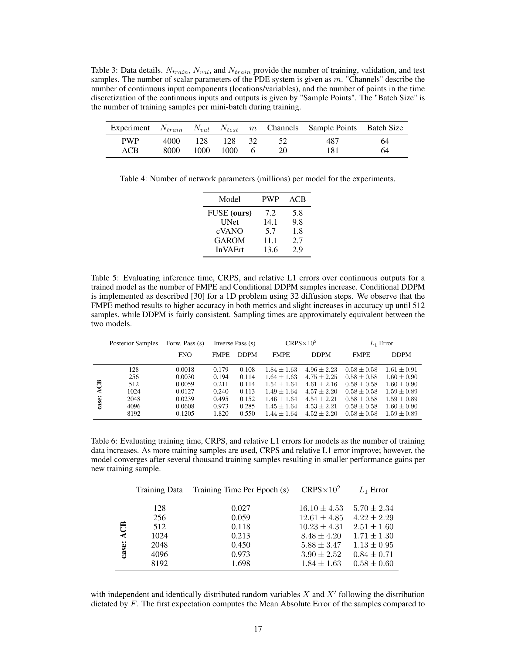
Table 4: Number of network parameters (millions) per model for the experiments.

🔼 This table presents a comparison of the performance of the proposed FUSE model against several baseline models in two tasks: estimating parameters (ξ) from continuous inputs (u) and predicting time series data (s). The performance is evaluated using three metrics: CRPS (Continuous Ranked Probability Score) for parameter estimation, and relative L1 and L2 errors for time series prediction. The table shows results for three levels of input information, representing varying levels of data completeness. ‘True parameters’ refers to the evaluation of only the forward model, while ‘Estimated parameters’ shows results of the unified forward-inverse model.
read the caption
Table 1: Performance of FUSE and the baseline models in estimating parameters ξ from continuous inputs u, quantified by CRPS, and predicting time series data s, quantified by a relative L₁ and L₂ error. Here, 'True parameters' evaluates the forward model part only, and 'Estimated parameters' and levels one to three evaluates the sample mean s predicted by the unified model.

🔼 This table presents a comparison of the performance of the proposed FUSE model against several baseline models in two tasks: estimating parameters from continuous inputs and predicting time series data. The metrics used for evaluation are CRPS (Continuous Ranked Probability Score) for parameter estimation and relative L1 and L2 errors for time series prediction. The table shows results for three different levels of input information, demonstrating the model’s performance under varying data availability.
read the caption
Table 1: Performance of FUSE and the baseline models in estimating parameters ξ from continuous inputs u, quantified by CRPS, and predicting time series data s, quantified by a relative L₁ and L2 error. Here, 'True parameters' evaluates the forward model part only, and 'Estimated parameters' and levels one to three evaluates the sample mean Predicted by the unified model.
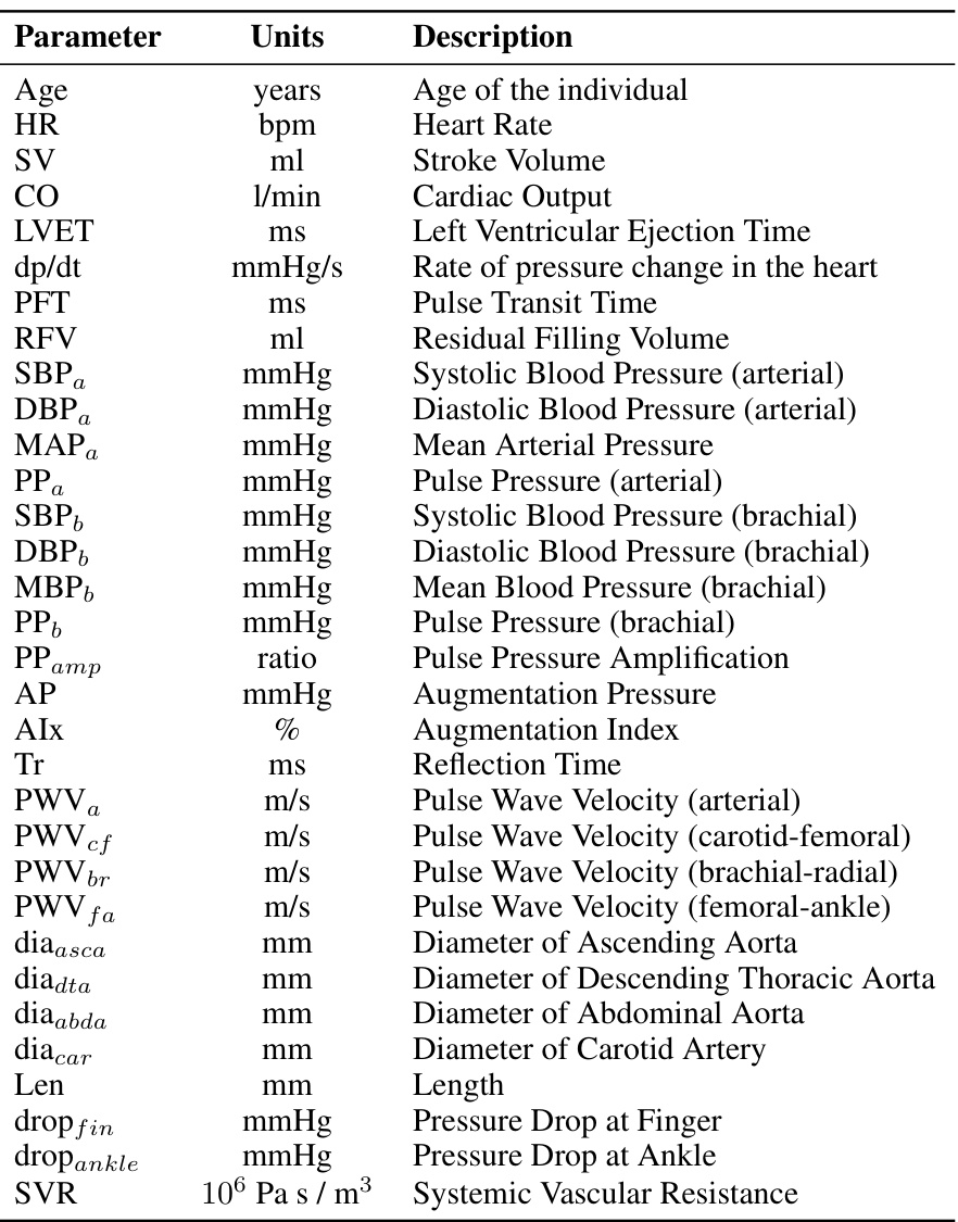
🔼 This table presents a comparison of the performance of the proposed FUSE model against several baseline models in two tasks: estimating parameters (ξ) from continuous inputs (u) and predicting time series data (s). The performance is measured using the Continuous Ranked Probability Score (CRPS) for parameter estimation and relative L₁ and L₂ errors for time series prediction. The table also breaks down the results for different levels of input information available.
read the caption
Table 1: Performance of FUSE and the baseline models in estimating parameters ξ from continuous inputs u, quantified by CRPS, and predicting time series data s, quantified by a relative L₁ and L₂ error. Here, 'True parameters' evaluates the forward model part only, and 'Estimated parameters' and levels one to three evaluates the sample mean s predicted by the unified model.
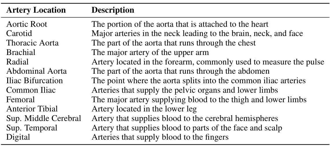
🔼 This table summarizes the performance comparison between FUSE and several baseline models in two tasks: estimating parameters (ξ) from continuous inputs (u) and predicting time series data (s). The parameter estimation performance is measured using the Continuous Ranked Probability Score (CRPS), while the prediction accuracy is assessed using relative L1 and L2 errors. The table also shows separate results for the ‘True Parameters’ (evaluating the forward model only) and ‘Estimated Parameters’ (using the full, unified FUSE model) across three different levels of input information.
read the caption
Table 1: Performance of FUSE and the baseline models in estimating parameters ξ from continuous inputs u, quantified by CRPS, and predicting time series data s, quantified by a relative L₁ and L₂ error. Here, 'True parameters' evaluates the forward model part only, and 'Estimated parameters' and levels one to three evaluates the sample mean Predicted by the unified model.
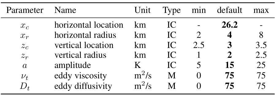
🔼 This table shows the discrete parameters used for the atmospheric cold bubble (ACB) experiment. It lists the parameter name, units, type (initial condition or model parameter), minimum value, default value, and maximum value used for sampling the training data. The horizontal location is fixed to maintain horizontal symmetry.
read the caption
Table 9: ACB: Discrete parameters with their ranges used for uniform sampling of the training data, as well as default values used by [56]. The parameters either encode the initial condition (IC) or are part of the sub-grid scale (SGS) model (M). The horizontal location x is kept fixed to ensure the horizontal symmetry of the domain.
Full paper#

