TL;DR#
Analyzing functional data, especially with noise and phase variability (variations in timings of events), is challenging. Current methods struggle to disentangle these variations from additive measurement errors, hindering accurate estimation of the fixed effect function (the average pattern). This research highlights the limitations of current techniques in reliably recovering this function due to these confounded variations.
The proposed solution is a new Bayesian model focused on the inherent geometric properties—size and shape—of the fixed effect function. Instead of directly modeling function values, it utilizes isometric actions that are invariant to phase variations. This allows reliable recovery of the size and shape. The model is regularized using informative priors, producing better estimates of the function’s geometry compared to existing methods. This addresses a critical issue, significantly improving the reliability of functional data analysis.
Key Takeaways#
Why does it matter?#
This paper is important because it presents a novel Bayesian functional mixed model that addresses the limitations of existing methods in analyzing functional data with phase variation. It offers a robust and reliable way to recover the size-and-shape of a fixed effect function, which has significant implications for various fields dealing with complex functional data. The use of size-and-shape preserving transformations opens new avenues for further research in this domain and offers a more geometrically intuitive approach to functional data analysis.
Visual Insights#

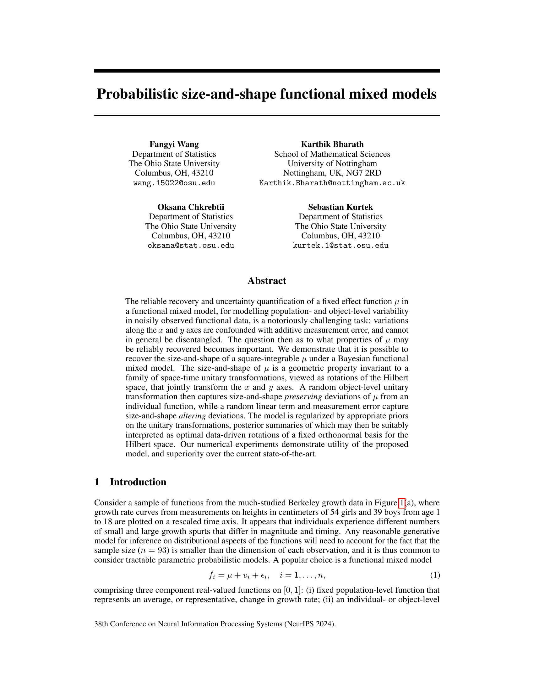
🔼 This figure shows examples of growth rate curves, phase functions and their transformations, and examples of PQRST complexes from electrocardiogram data. Panel (a) shows the Berkeley growth data, which consists of height measurements of children over time. Panel (b) is an example of a convex phase function, which is a function that maps time to time in a non-linear way. Panels (c), (d), and (e) show different transformations of the growth curves in (a), the PQRST complexes from ECG data, and an example PQRST pattern, respectively.
read the caption
Figure 1: (a) Berkeley growth rate curves. (b) Convex phase function γ. (c) One example function f from (a) (blue) transformed by value-preserving action foγ (red) and norm-preserving action (for)√y (yellow). Here, foy has the same classical notion of shape as f, whereas (for)√y has the same size-and-shape as f as described in Section 2. (d) PQRST complexes. (e) PQRST pattern: P wave (first max), QRS complex (sharp min-max-min) and T wave (last max) [Pham et al., 2023].

🔼 This table compares the accuracy of estimating the fixed effect (μ) using four different Bayesian models and the warpMix method. The accuracy is measured by the estimation error, which is calculated for three different functions (μ₁, μ₂, μ₃). The table highlights the model with the lowest estimation error for each function, demonstrating that the proposed Bayesian models often outperform warpMix.
read the caption
Table 1: Comparison of fixed effect estimation accuracy based on posterior mean from proposed Bayesian models and warpMix estimate. Smallest estimation errors are highlighted in bold.
In-depth insights#
Size-Shape Models#
Size-shape models offer a powerful paradigm for analyzing data where both size and shape are important, but confounded. They elegantly decouple these aspects, allowing for a more nuanced understanding of variability and relationships. This is particularly useful in scenarios with noisy or incomplete data, where traditional methods struggle. By focusing on shape, often represented as a set of landmarks or a curve, while accounting for size through scaling or other transformations, these models are robust to certain types of variation. Applications span diverse fields, including medical imaging, biology, and computer vision, where understanding the shape of an object (e.g., a tumor, organ, or object in an image) regardless of its size is crucial for diagnosis, classification, or analysis. The use of geometric or group-theoretic frameworks provide a mathematical rigor and elegance, enabling efficient analysis and inference. However, model complexity, computational cost, and the choice of appropriate shape representation can pose challenges, requiring careful consideration of the specific application and data.
Bayesian Inference#
Bayesian inference, in the context of a research paper on probabilistic size-and-shape functional mixed models, would likely involve specifying prior distributions for the model parameters (fixed effects, random effects, and hyperparameters). These priors encode prior beliefs or knowledge about the parameters before observing data. The model then updates these priors based on observed data through Bayes’ theorem, yielding posterior distributions that reflect a synthesis of prior knowledge and observed evidence. The choice of priors is crucial and should be justified. Markov Chain Monte Carlo (MCMC) methods are likely used to sample from the complex, high-dimensional posterior distributions, especially if closed-form solutions are not available. The paper would then present posterior summaries (e.g., means, credible intervals) for the parameters of interest, along with diagnostic checks for MCMC convergence and model adequacy. In the application to functional data, the Bayesian framework’s capacity to handle uncertainty quantification would be a key strength, offering insights beyond traditional frequentist approaches by providing a measure of uncertainty associated with model estimates.
Phase Variation#
Phase variation in functional data analysis refers to variations in the timing or phase of features within functions. This is distinct from amplitude variation, which concerns the magnitude of the features. Modeling phase variation is challenging because it’s often confounded with amplitude variations and measurement error, making it difficult to isolate and interpret. Approaches to handle phase variation include registration techniques, which aim to align functions based on their features, allowing for better comparison and analysis. Bayesian methods offer a powerful framework for modeling uncertainty associated with phase variation by introducing priors to constrain the variability of phase functions. The effectiveness of a chosen approach for handling phase variation is crucial for accurately analyzing data with such variation, as the choice can significantly impact results such as the estimation of the population-level mean function.
Model Comparison#
A robust model comparison section in a research paper is crucial for establishing the validity and superiority of a proposed model. It should go beyond simply stating performance metrics. A strong comparison should involve multiple baselines, reflecting the current state-of-the-art and including methods with similar assumptions or goals. The selection of these baselines should be justified. Quantitative comparisons using metrics relevant to the model’s aims (e.g., accuracy, precision, recall, F1-score for classification; RMSE, MAE for regression; log-likelihood for probabilistic models) are essential. However, these should be complemented by qualitative analysis. For example, visualisations may reveal patterns or characteristics not immediately apparent in numbers. A discussion of the computational cost of each method is vital for practical applications, highlighting the trade-off between model complexity and performance. Furthermore, a detailed analysis of the factors contributing to differences in model performance, such as dataset characteristics or hyperparameter choices, provides a deeper understanding. Finally, limitations of both the proposed and baseline models should be acknowledged, providing a balanced perspective on the findings. Only through such a comprehensive comparison can the true value and limitations of the proposed model be effectively evaluated.
Future Work#
Future research directions stemming from this work could explore several avenues. Extending the model to handle higher-dimensional data (e.g., images or 3D shapes) would broaden its applicability. Investigating alternative prior distributions for the phase functions and developing more efficient inference algorithms (beyond MCMC) would improve scalability and computational efficiency. Rigorous theoretical analysis establishing convergence rates and uncertainty quantification would enhance the model’s reliability. Finally, application to diverse datasets across various domains (biomedical, environmental, etc.) will demonstrate the model’s generalizability and uncover new insights. Addressing the impact of hyperparameter choices on model performance is another important direction for future investigation. A careful analysis could aid the development of data-driven methods for hyperparameter selection or optimization.
More visual insights#
More on figures
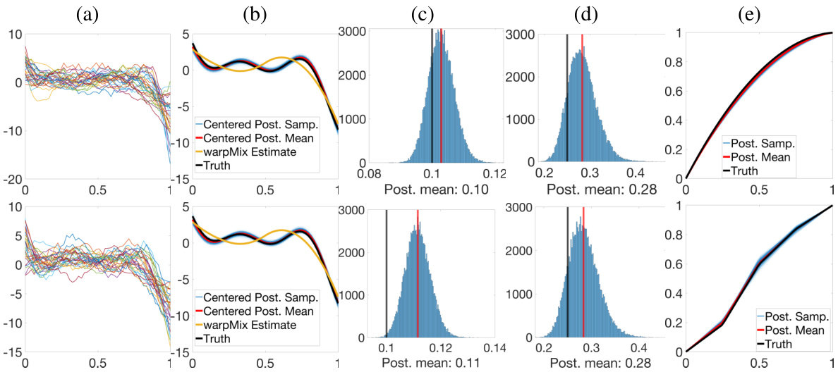
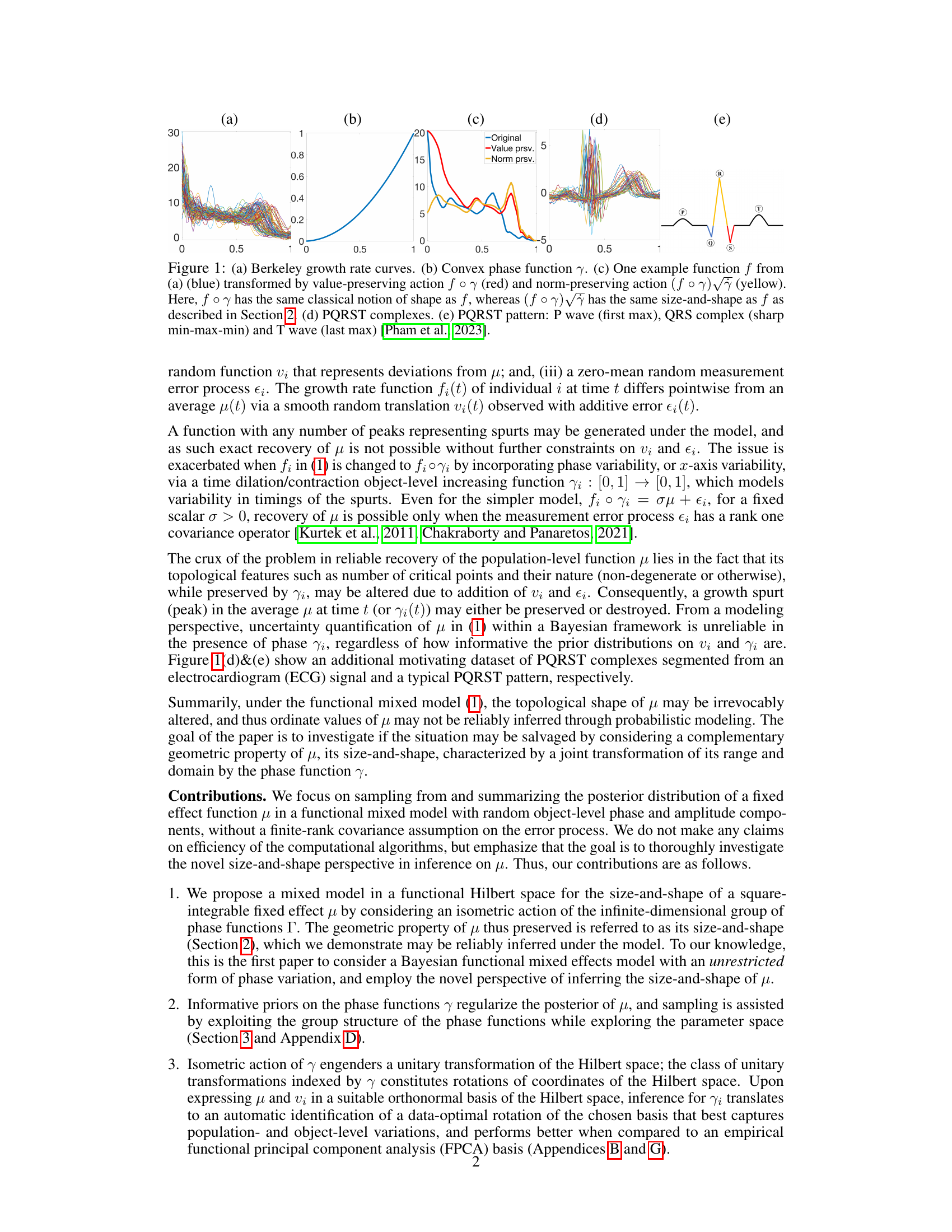
🔼 This figure shows the results of a simulation study using two different prior models for phase functions (PM1 and PM2). Panel (a) displays the simulated data. Panel (b) compares the estimation of the fixed effect function μ using the proposed Bayesian model (posterior samples and mean) and the warpMix model. Panels (c) and (d) show the posterior distributions of the variance parameters σ² and σe². Finally, panel (e) presents the estimation results for a randomly chosen phase function.
read the caption
Figure 2: Row 1: Phase functions from PM1. Row 2: Phase functions from PM2. (a) Simulated data (n = 30). (b) Estimation of μ: ground truth (black), posterior samples (blue), posterior mean (red), warpMix esimate (yellow). (c)&(d) Histograms of posterior samples for σ² and σ², respectively (posterior mean in red; ground truth in black). (e) Estimation of phase function for a randomly chosen observation: ground truth (black), posterior samples (blue), posterior mean (red).

🔼 This figure compares the estimation results of the proposed Bayesian model (Model 2-B) and the warpMix method for three different fixed effect functions (μ₁, μ₂, μ₃). The ground truth function is shown in black, the centered posterior samples from the Bayesian model are shown in blue, the centered posterior mean is shown in red, and the warpMix estimate is shown in yellow. The figure visually demonstrates the effectiveness of the proposed Bayesian model in capturing the properties of the fixed effect functions, especially in comparison to the warpMix method.
read the caption
Figure 3: Comparison of estimation results based on Model 2-B and warpMix for (a) μ₁, (b) μ2 and (c) μ3. In each panel, we show the ground truth (black), centered posterior samples (blue), centered posterior mean (red), and warpMix estimate (yellow).
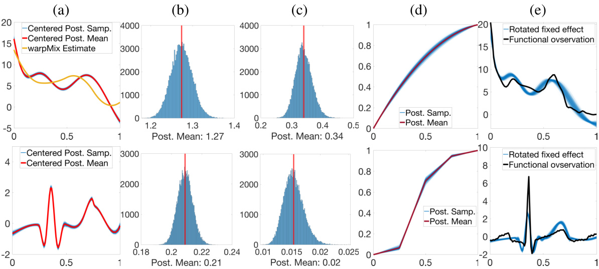
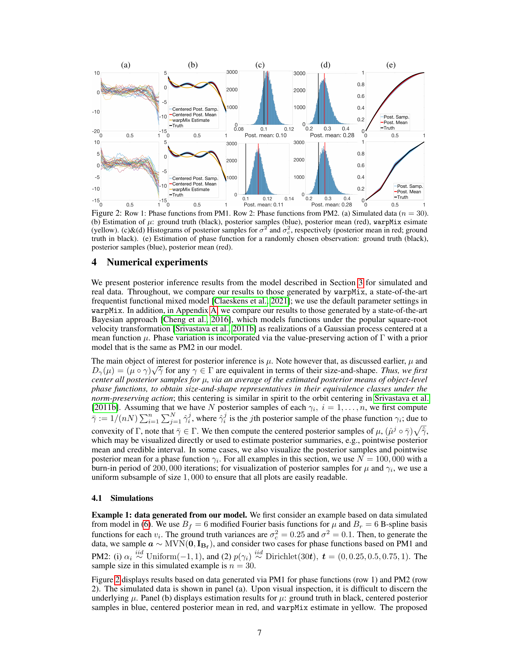
🔼 This figure shows the results of applying the proposed Bayesian model to the Berkeley growth data and PQRST complexes. The first row shows the results for the Berkeley growth data, while the second row shows the results for the PQRST complexes. The figure includes plots of the posterior samples and posterior mean of μ, histograms of the posterior samples of σ² and σe, a plot of the posterior samples and mean of the phase function for a randomly chosen observation, and a plot showing the observation corresponding to the phase function along with rotated posterior samples of μ. The warpMix model was unable to yield an estimate of μ for the PQRST data.
read the caption
Figure 4: Estimation results for Berkeley data (row 1) and PQRST complexes (row 2). (a) Posterior samples (blue) and posterior mean (red) of μ, and warpMix estimate (yellow). The warpMix model was unable to yield an estimate of μ for PQRST data. (b)&(c) Histograms of posterior samples for σ² and σ², respectively (posterior mean in red). (d) Posterior samples (blue) and mean (red) of phase function for a randomly chosen observation. (e) Observation corresponding to (d) (black) with rotated posterior samples of μ (blue).

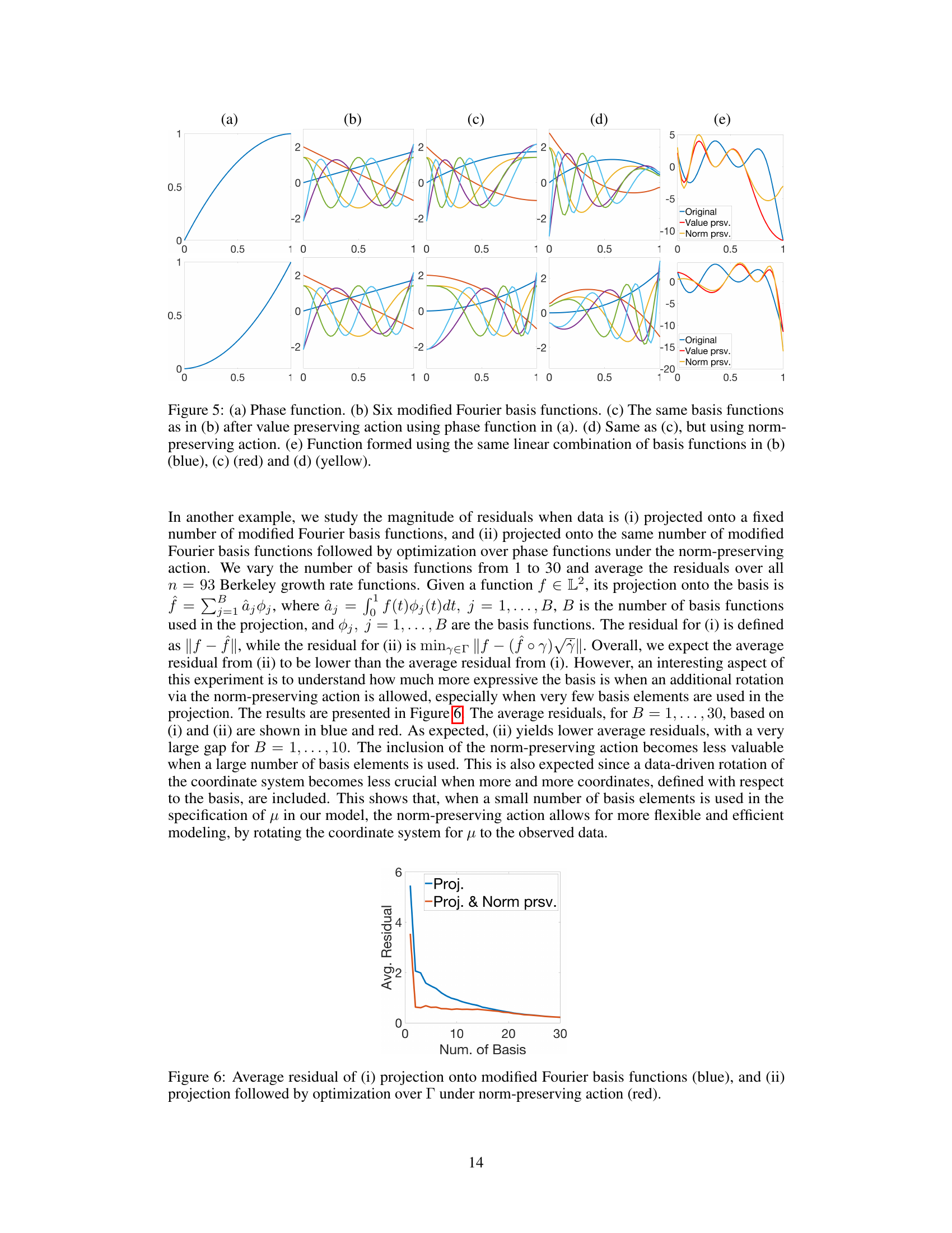
🔼 This figure compares the value-preserving and norm-preserving actions on a set of basis functions. Panel (a) shows an example phase function. Panels (b), (c), and (d) show six modified Fourier basis functions, the same functions after the value-preserving transformation, and the same functions after the norm-preserving transformation, respectively. Panel (e) illustrates how these transformations affect a function formed from a linear combination of these basis functions. The norm-preserving transformation creates a function with a different shape, while the value-preserving transformation mostly shifts or scales the function, preserving the overall shape.
read the caption
Figure 5: (a) Phase function. (b) Six modified Fourier basis functions. (c) The same basis functions as in (b) after value preserving action using phase function in (a). (d) Same as (c), but using norm-preserving action. (e) Function formed using the same linear combination of basis functions in (b) (blue), (c) (red) and (d) (yellow).

🔼 This figure shows the average residual error when projecting the Berkeley growth data onto modified Fourier basis functions. The blue line represents the average residual when only projecting onto the basis functions. The red line shows the average residual when additionally performing optimization over the phase functions using the norm-preserving action. The results demonstrate that including the norm-preserving action significantly reduces the residual, especially when a small number of basis functions are used.
read the caption
Figure 6: Average residual of (i) projection onto modified Fourier basis functions (blue), and (ii) projection followed by optimization over Γ under norm-preserving action (red).
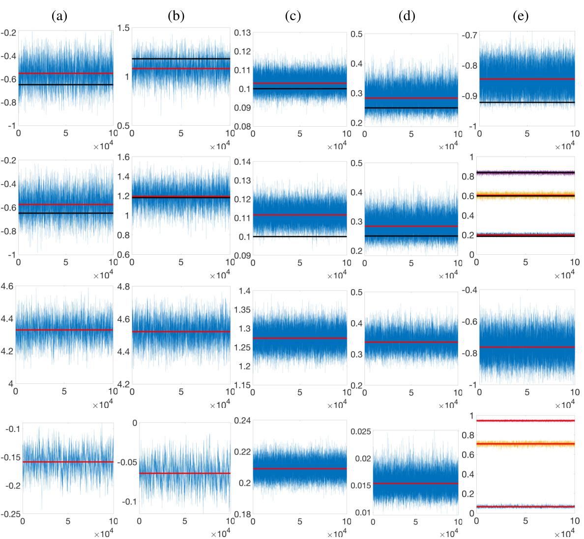
🔼 This figure displays MCMC diagnostic plots for all model parameters, including the fixed-effect coefficients, error variance, variance of size-and-shape altering random effects, and the size-and-shape preserving random effect (phase function). It shows trace plots for four different datasets: two simulated datasets and two real-world datasets (Berkeley growth data and PQRST complexes). The plots illustrate the convergence of the MCMC algorithm towards the stationary posterior distribution for each parameter, comparing the posterior mean to the ground truth where applicable.
read the caption
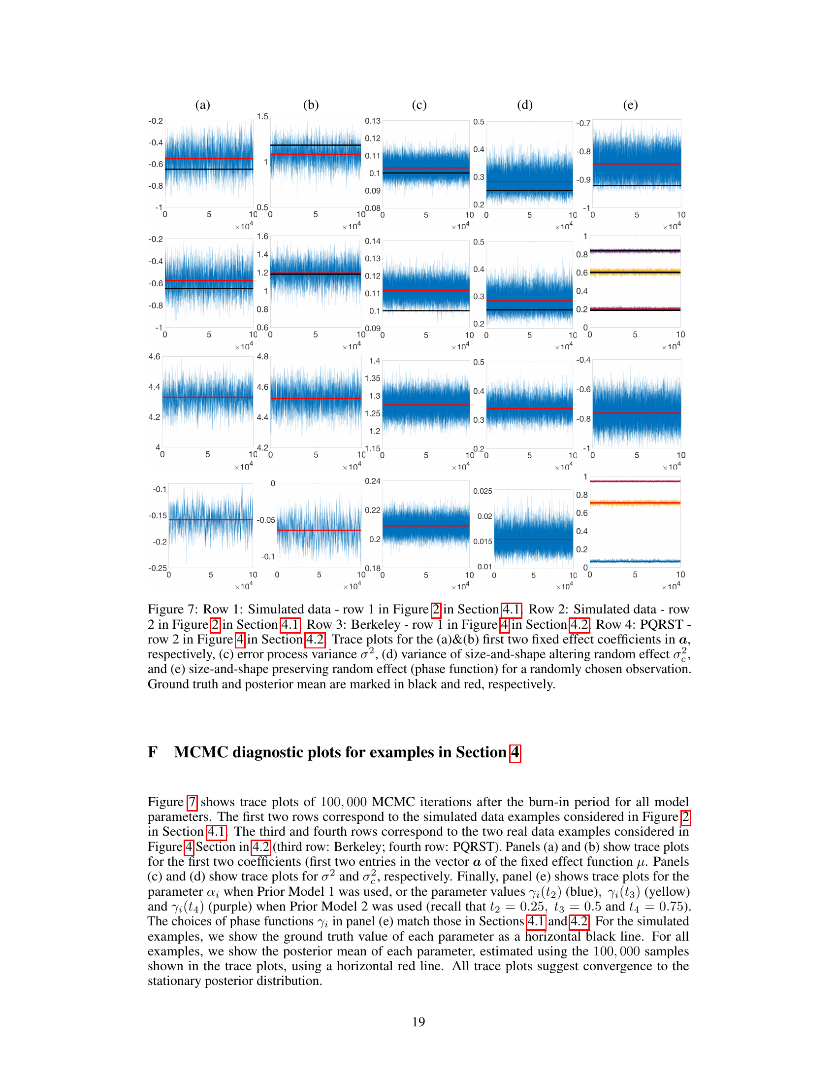
Figure 7: Row 1: Simulated data - row 1 in Figure 2 in Section 4.1. Row 2: Simulated data - row 2 in Figure 2 in Section 4.1. Row 3: Berkeley - row 1 in Figure 4 in Section 4.2. Row 4: PQRST - row 2 in Figure 4 in Section 4.2. Trace plots for the (a)&(b) first two fixed effect coefficients in a, respectively, (c) error process variance σ², (d) variance of size-and-shape altering random effect σ², and (e) size-and-shape preserving random effect (phase function) for a randomly chosen observation. Ground truth and posterior mean are marked in black and red, respectively.
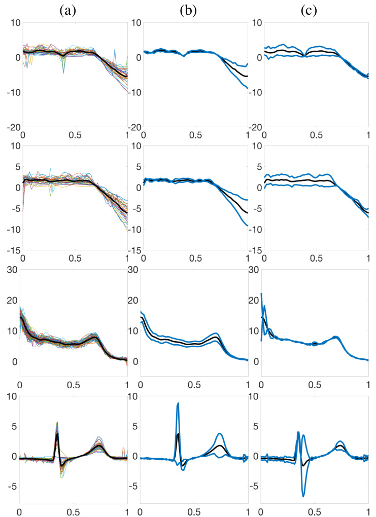
🔼 This figure compares the results of the proposed Bayesian model and the warpMix model for five real-world datasets. Each dataset’s raw data is shown, followed by the estimated posterior mean and 95% credible interval of the fixed effect function (μ) using both Prior Models 1 and 2 for the phase functions. The warpMix estimate of μ is also included for comparison. The figure illustrates how well the Bayesian model recovers the underlying patterns in the data, even with variations in magnitude and timing.
read the caption
Figure 11: Estimation results for the pinch force, respiration, gait, signature acceleration and gene expression datasets (top to bottom). (a) Data. (b)&(c) Centered posterior mean (black) and 95% credible interval (dashed blue) for μ when Prior Models 1 and 2 are used for phase functions, respectively. (d) warpMix estimate.
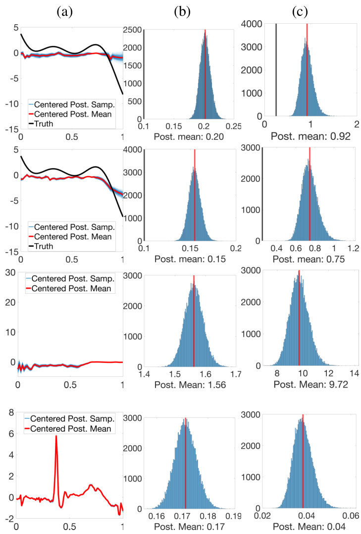
🔼 Figure 2 presents the results of applying the proposed Bayesian model to simulated data. The first row shows results for the first prior model (PM1) while the second row shows results for the second prior model (PM2). Panel (a) shows the simulated data. Panel (b) compares the estimated fixed-effect function (μ) to the ground truth showing the posterior samples and mean, as well as the estimate from the warpMix method. Panels (c) and (d) show the posterior distributions for the variance parameters and their means. Finally, panel (e) shows the estimation results for the phase function for a randomly chosen observation.
read the caption
Figure 2: Row 1: Phase functions from PM1. Row 2: Phase functions from PM2. (a) Simulated data (n = 30). (b) Estimation of μ: ground truth (black), posterior samples (blue), posterior mean (red), warpMix esimate (yellow). (c)&(d) Histograms of posterior samples for σ² and σ², respectively (posterior mean in red; ground truth in black). (e) Estimation of phase function for a randomly chosen observation: ground truth (black), posterior samples (blue), posterior mean (red).
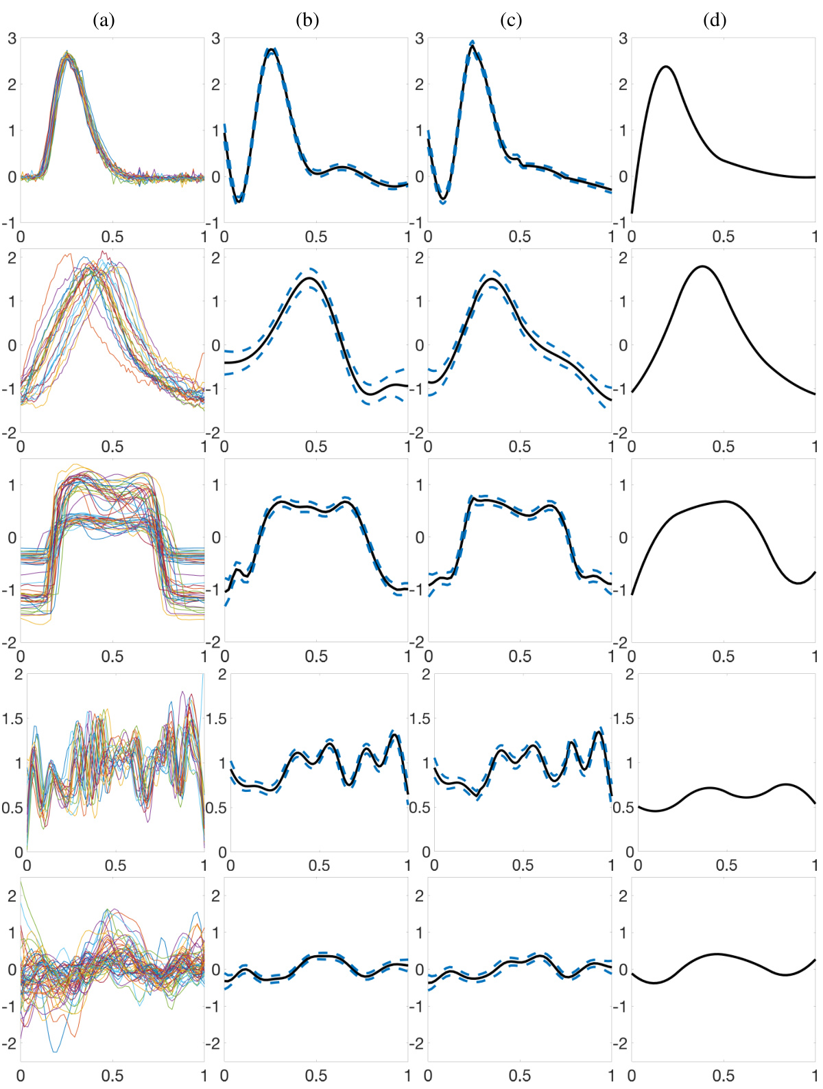
🔼 This figure shows the estimation results of the proposed Bayesian model for five real datasets. The first row shows the raw data for each dataset. The second and third rows show the posterior mean and 95% credible interval of the size-and-shape of μ for the models using Prior Model 1 and Prior Model 2, respectively. The last row shows the results of warpMix model. The results demonstrate that the proposed model can effectively recover the size-and-shape of μ in various real datasets.
read the caption
Figure 11: Estimation results for the pinch force, respiration, gait, signature acceleration and gene expression datasets (top to bottom). (a) Data. (b)&(c) Centered posterior mean (black) and 95% credible interval (dashed blue) for μ when Prior Models 1 and 2 are used for phase functions, respectively. (d) warpMix estimate.
Full paper#
