TL;DR#
Offline Reinforcement Learning (RL) faces challenges with handling out-of-distribution data and noisy labels, especially when using transformer-based models. Existing approaches struggle to fully utilize historical temporal information and intra-step relationships among states, actions, and rewards. They also tend to overfit suboptimal trajectories with noisy labels.
To overcome these limitations, the paper introduces Decision Mamba (DM), a multi-grained SSM with a self-evolving policy learning strategy. DM models historical hidden states using a mamba architecture to capture temporal information and employs a fine-grained SSM module to capture intra-step relationships. A self-evolving policy, using progressive regularization, enhances robustness to noise. Empirical results on benchmark tasks showcase DM’s substantial performance improvements over existing methods.
Key Takeaways#
Why does it matter?#
This paper is crucial for researchers in offline reinforcement learning because it addresses the critical issue of handling out-of-distribution states and actions, a major limitation of existing transformer-based methods. By introducing a novel multi-grained state space model and a self-evolving policy learning strategy, the study significantly improves the robustness and performance of offline RL algorithms. This opens up new avenues for research by combining the strengths of SSMs and transformers for offline RL, paving the way for more reliable and effective solutions in real-world applications.
Visual Insights#

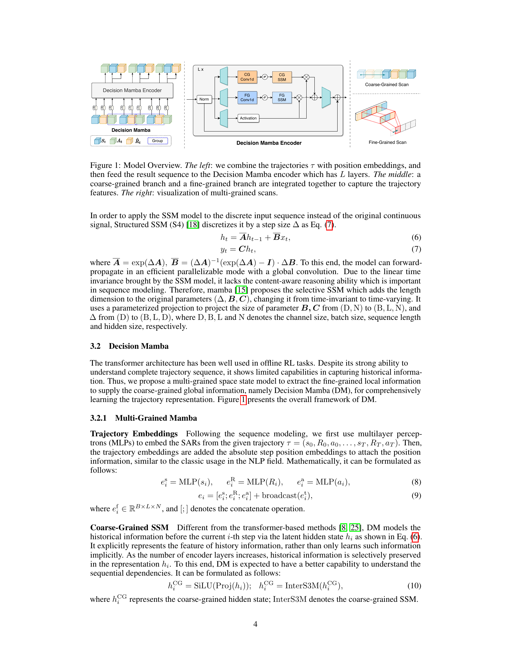
🔼 This figure provides a high-level overview of the Decision Mamba model architecture. The left panel shows the input processing stage, where trajectories are combined with positional embeddings and fed into the encoder. The middle panel details the encoder’s core structure, highlighting the integration of coarse-grained and fine-grained branches to capture both global and local trajectory features. The right panel illustrates the concept of multi-grained scans, visualizing how both global and local features are extracted and processed within the architecture.
read the caption
Figure 1: Model Overview. The left: we combine the trajectories T with position embeddings, and then feed the result sequence to the Decision Mamba encoder which has L layers. The middle: a coarse-grained branch and a fine-grained branch are integrated together to capture the trajectory features. The right: visualization of multi-grained scans.

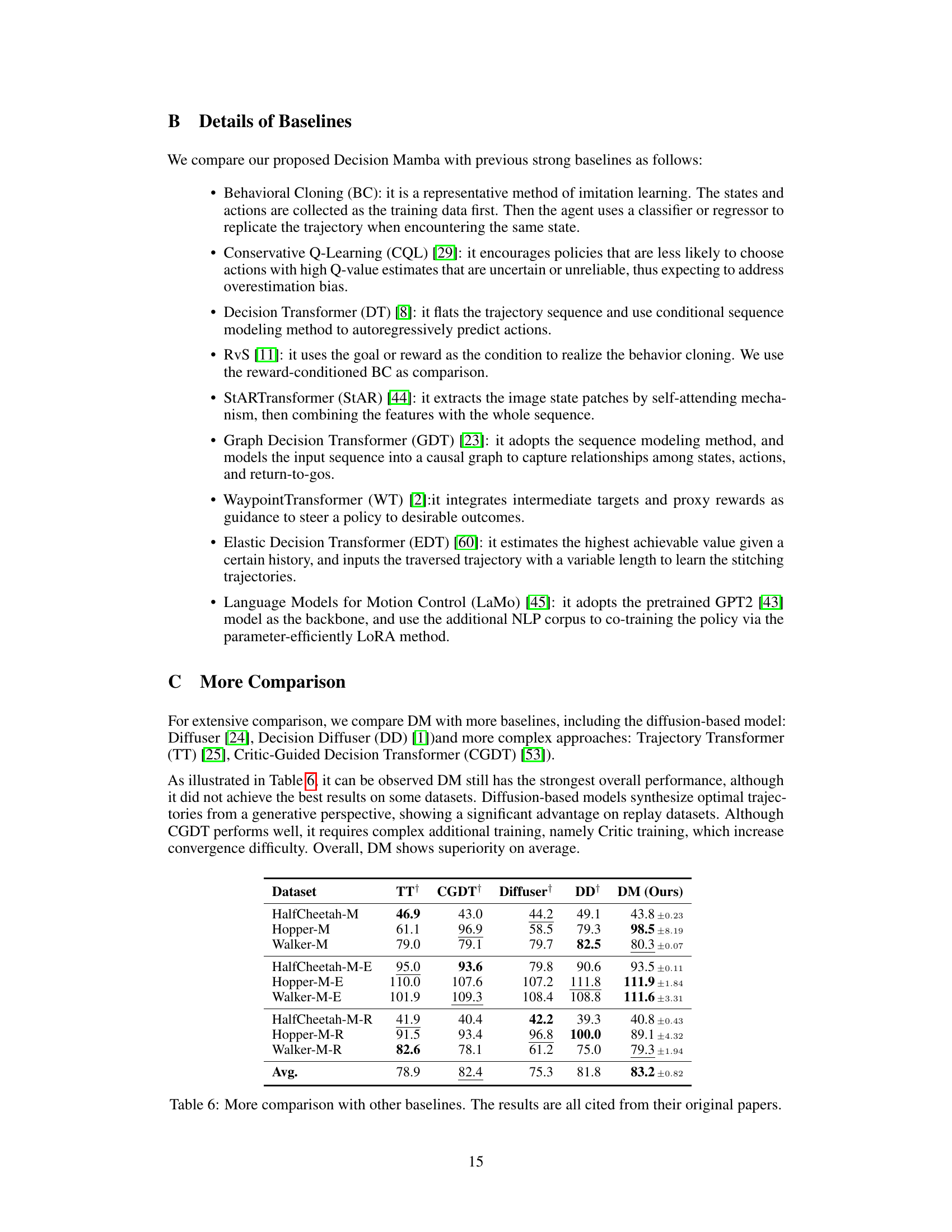
🔼 This table presents the overall performance comparison of Decision Mamba (DM) against various baseline offline reinforcement learning methods across different datasets (medium, medium-expert, and medium-replay). The performance is measured by the normalized score, averaged over four runs with different random seeds. The best and second-best results for each dataset are highlighted.
read the caption
Table 1: Overall Performance. M, M-E, and M-R denotes the medium, medium-expert, and medium-replay, respectively. The results of the baselines marked with † are cited from their original papers. We report the mean and standard deviation of the normalized score with four random seeds. Bold and underline indicate the highest score and second-highest score, respectively.
In-depth insights#
Offline RL via SSM#
Offline reinforcement learning (RL) presents unique challenges due to the absence of an interactive environment. State Space Models (SSMs) offer a compelling alternative to traditional methods by explicitly modeling the system’s hidden state and dynamics. This approach allows for efficient representation of temporal dependencies in offline data, which is crucial for accurate policy learning. SSMs excel at handling long-range dependencies and complex sequential patterns often found in offline RL datasets, enabling better generalization and robustness. However, effectively leveraging SSMs in offline RL requires careful consideration of model design and training strategies to overcome challenges such as noisy data and overfitting. Addressing issues like model complexity and computational efficiency will further unlock the potential of SSMs to advance the state-of-the-art in offline RL.
Multi-grained Mamba#
The proposed “Multi-grained Mamba” architecture represents a novel approach to offline reinforcement learning by integrating both coarse-grained and fine-grained state space models (SSMs). This dual-level approach is designed to effectively capture both the global temporal dynamics of a trajectory (coarse-grained) and the intricate local relationships among states, actions, and rewards within each time step (fine-grained). The coarse-grained SSM leverages the historical temporal information to effectively extract the sequential patterns, while the fine-grained SSM focuses on uncovering the intricate causal relationships at the intra-step level. This integration of different SSM scales allows the model to learn more comprehensive trajectory representations, potentially improving the robustness of decision-making in offline settings, especially when facing noisy or incomplete data. By combining these aspects, the model is able to gain a more detailed representation of both global trajectory patterns and local dynamics, allowing it to generate better decision outcomes. The integration within the Mamba architecture further enhances the efficiency and effectiveness of this multi-scale modeling technique.
Self-evolving Policy#
A self-evolving policy is a machine learning model that iteratively improves its own decision-making process. Instead of relying solely on a fixed set of training data, it uses its past experience and performance to refine its strategies over time. This approach offers several advantages, such as enhanced robustness to noisy or incomplete data, adaptive learning in dynamic environments, and better generalization to unseen situations. A key aspect of a self-evolving policy is the mechanism by which it updates its internal representation. This often involves reinforcement learning algorithms that allow the model to learn from its successes and failures. However, designing an effective self-evolution mechanism requires careful consideration of several factors, including the model’s architecture, the learning rate, and the balance between exploration and exploitation. Overfitting is a significant risk, therefore regularization techniques are crucial to ensure that the model doesn’t become overly specialized to its past experiences. Overall, the use of self-evolving policies offers a powerful new paradigm for creating AI systems that can continuously learn and adapt.
Empirical Evaluation#
A robust empirical evaluation section should meticulously detail the experimental setup, including datasets used, metrics for assessment, and baseline algorithms compared against. Clear descriptions of the model’s hyperparameters and training procedures are essential for reproducibility. The results should be presented systematically, possibly using tables and graphs for easy interpretation, and statistical significance should be rigorously addressed to avoid spurious conclusions. Comparing the proposed method against multiple established baselines, rather than just one or two, strengthens the evaluation. The analysis of the results should extend beyond simply reporting performance metrics; it should also explore the model’s behavior under various conditions and provide insights into its strengths and weaknesses. A thoughtful discussion of unexpected results and limitations is also crucial for demonstrating a thorough and insightful empirical evaluation.
Future Work#
Future research directions stemming from this Decision Mamba model could involve several key areas. Extending the model to handle continuous action spaces would broaden its applicability to a wider range of real-world problems. Currently, the model is tailored for discrete actions; continuous adaptation would significantly enhance its practical use. Investigating more sophisticated regularization techniques beyond the progressive self-evolution method could further improve robustness and mitigate overfitting on noisy data. Exploring alternative regularization methods, or combining them with the current approach, is worth investigating. Incorporating uncertainty estimation into the model’s predictions would be valuable, allowing for more informed decision-making in situations with inherent stochasticity. This could involve Bayesian methods or other approaches to quantify uncertainty. Finally, evaluating the model’s performance on more complex and diverse tasks beyond those in the benchmark datasets is crucial for assessing its true capabilities and generalizability.
More visual insights#
More on figures

🔼 This figure provides a high-level overview of the Decision Mamba model architecture. It shows three key components: the trajectory embedding process (left), the multi-grained state space model (SSM) which combines coarse-grained and fine-grained information (middle), and a visualization of the multi-grained scanning mechanism (right). The left side illustrates how trajectories are processed using position embeddings and fed into the model’s encoder. The middle section details the core architecture of Decision Mamba, showing how it uses both coarse-grained and fine-grained SSMS to capture trajectory features at different scales. The right section shows the scanning method across different scales.
read the caption
Figure 1: Model Overview. The left: we combine the trajectories T with position embeddings, and then feed the result sequence to the Decision Mamba encoder which has L layers. The middle: a coarse-grained branch and a fine-grained branch are integrated together to capture the trajectory features. The right: visualization of multi-grained scans.
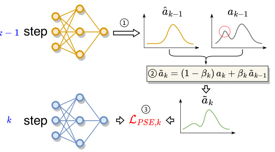
🔼 This figure illustrates the Progressive Self-Evolution Regularization (PSER) process. It shows three steps: 1) The previous step’s policy (k-1) generates action labels. 2) These labels are refined by combining them with the current policy’s predictions (k), using a weighted average controlled by βk. The weighting emphasizes the current step’s prediction when βk is closer to 0 and the previous step’s prediction when βk is close to 1. 3) The refined labels are then used to compute a loss function (LPSE,k), guiding the training process to focus more on clean data while mitigating the effects of noisy data points (represented by the red circle).
read the caption
Figure 2: The process of PSER includes: i) generating action labels with previous step policy, ii) refining target label, iii) computing loss, where the red circle denotes the noise.

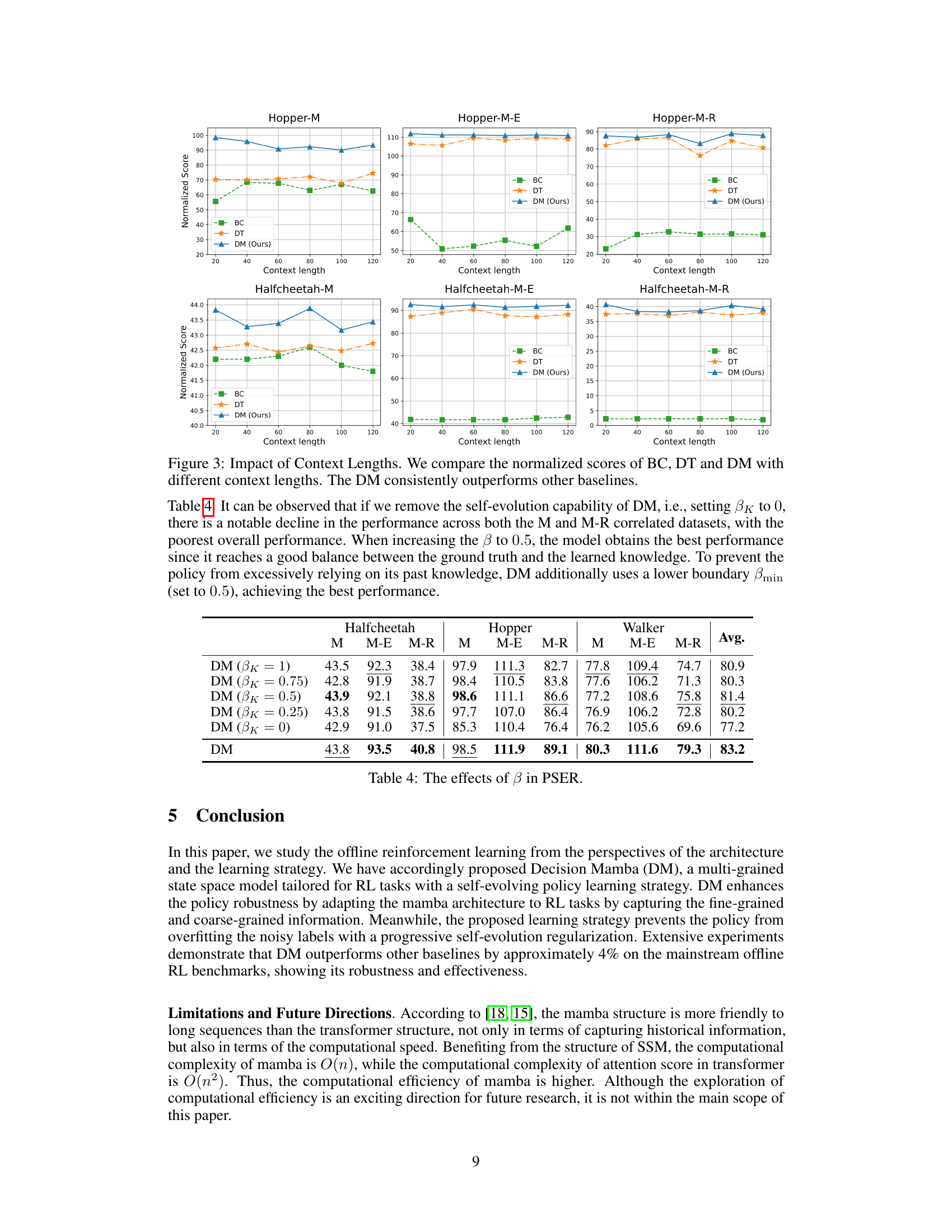
🔼 This figure shows the results of an experiment comparing the performance of three different offline reinforcement learning models (BC, DT, and DM) across various context lengths. The experiment was conducted on three different datasets (Hopper-M, Hopper-M-E, Hopper-M-R, Halfcheetah-M, Halfcheetah-M-E, Halfcheetah-M-R). The results demonstrate that the Decision Mamba (DM) model consistently outperforms the other two models across all datasets and context lengths, indicating its robustness and effectiveness in capturing both local and global information from the trajectory data. The y-axis represents the normalized score of each model, and the x-axis represents the length of the context window used in the model.
read the caption
Figure 3: Impact of Context Lengths. We compare the normalized scores of BC, DT and DM with different context lengths. The DM consistently outperforms other baselines.

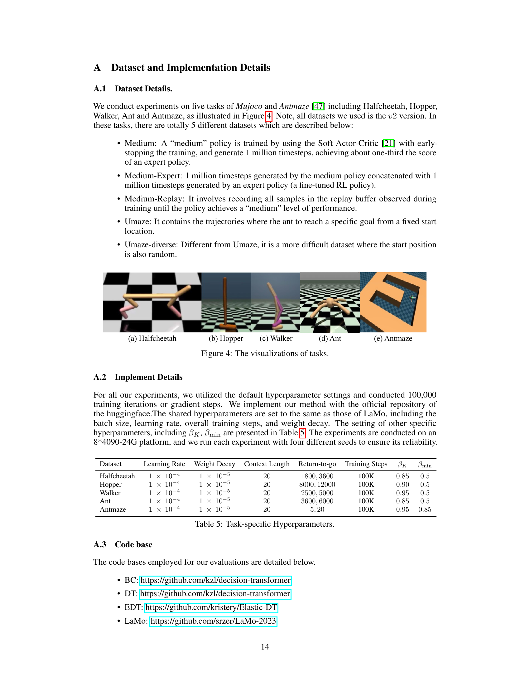
🔼 This figure visualizes the five different tasks used in the experiments: HalfCheetah, Hopper, Walker, Ant, and Antmaze. Each image shows a different robotic agent in its environment, highlighting the diversity of the tasks.
read the caption
Figure 4: The visualizations of tasks.

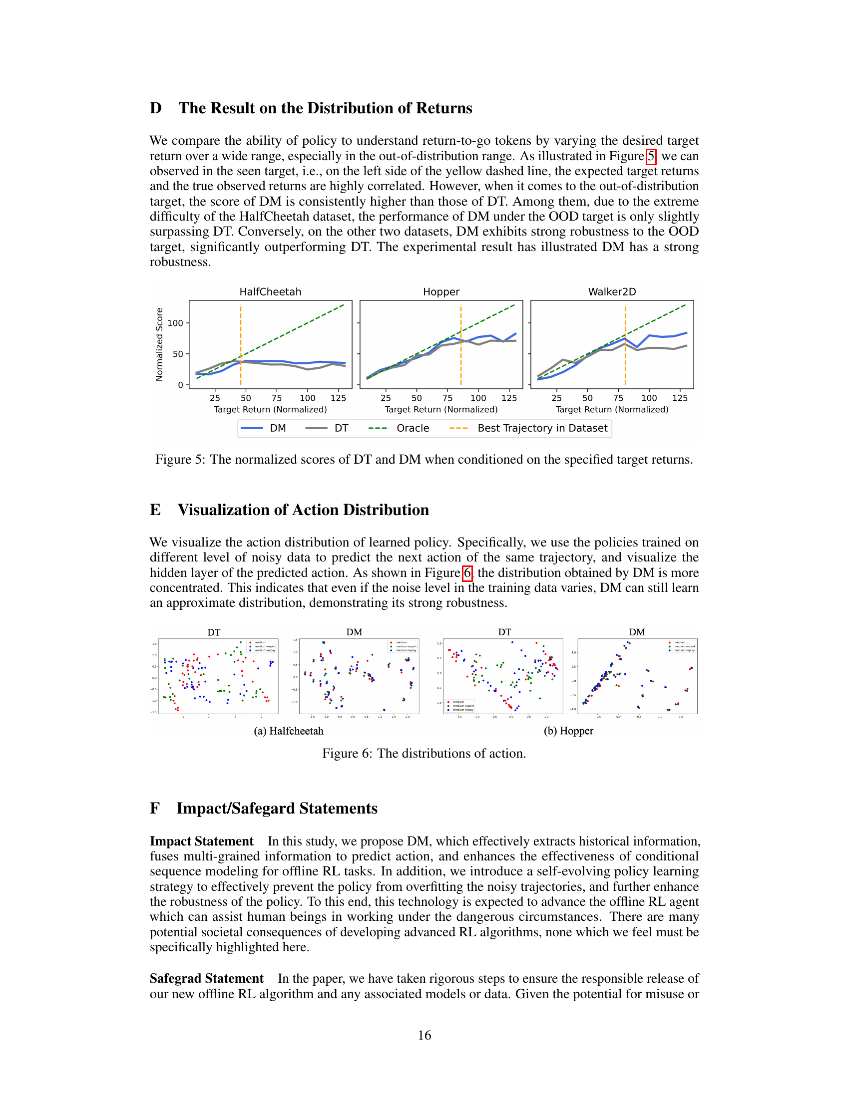
🔼 This figure compares the performance of Decision Transformer (DT) and Decision Mamba (DM) models when predicting actions based on different target returns. The x-axis represents the target return (normalized), and the y-axis represents the normalized score achieved by each model. The figure shows that DM consistently outperforms DT, especially in the out-of-distribution (OOD) region (returns beyond the range observed in the training data). The dashed lines represent the oracle (optimal) performance and the best trajectory in the training dataset. The results demonstrate that DM is more robust to unseen return-to-go values than DT.
read the caption
Figure 5: The normalized scores of DT and DM when conditioned on the specified target returns.

🔼 This figure visualizes the action distribution of the learned policies trained on different levels of noisy data. It shows the hidden layer of the predicted action to compare the action distribution learned by Decision Transformer (DT) and Decision Mamba (DM). DM’s distribution is more concentrated, indicating its robustness to varying noise levels in the training data.
read the caption
Figure 6: The distributions of action.
More on tables
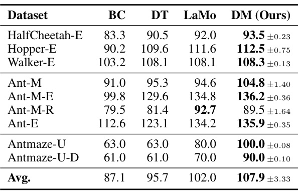
🔼 This table presents a comprehensive comparison of the performance of Decision Mamba (DM) against various baseline methods across different datasets with varying levels of difficulty. The datasets are categorized by their difficulty (Expert, Umazed, Umazed-Diverse) and the results are represented by average normalized scores. This allows for a robust evaluation of DM’s performance in offline reinforcement learning across diverse scenarios and quality levels of data.
read the caption
Table 2: Extensive Results. E, U, and U-D denotes the expert, umazed, and umazed-diverse.

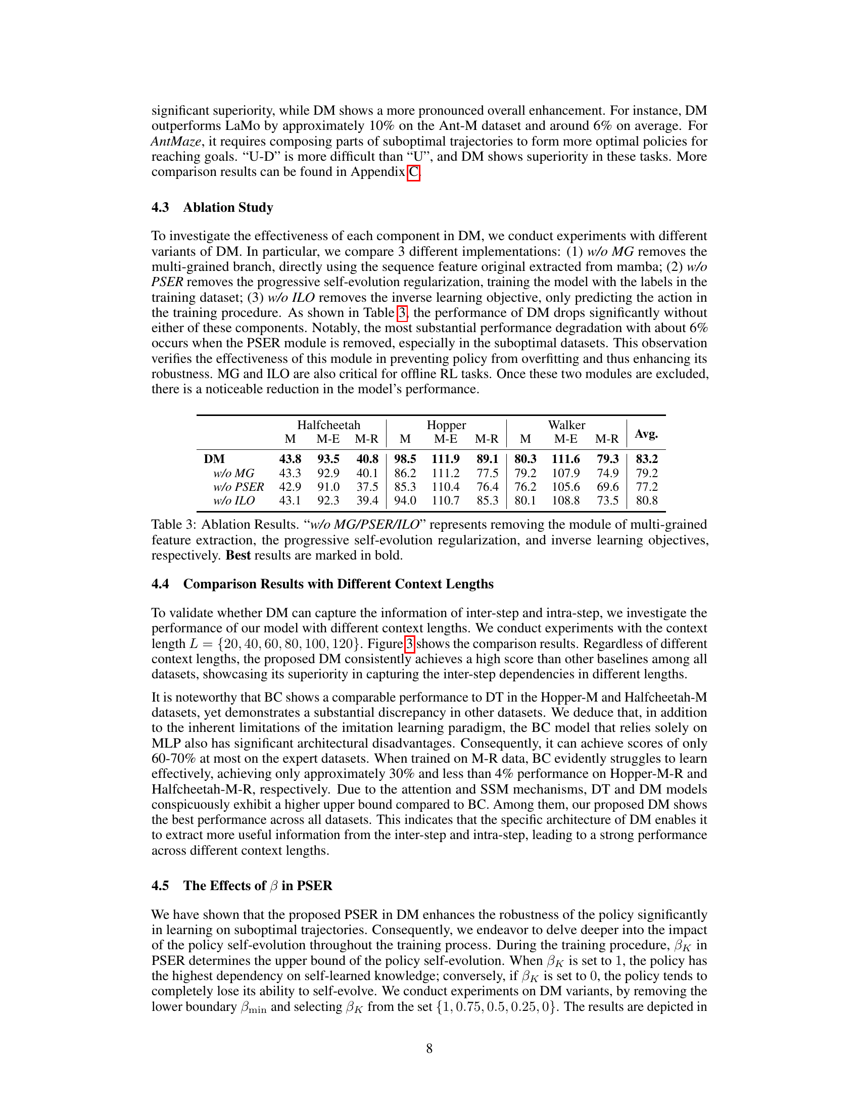
🔼 This table presents the ablation study results for the Decision Mamba model. It shows the impact of removing each of three key components: the multi-grained feature extraction, progressive self-evolution regularization, and inverse learning objective. The table compares the average performance across multiple metrics (Halfcheetah, Hopper, Walker, Avg) and different dataset difficulties (M, M-E, M-R) by showing the performance drop when each component is removed. The results demonstrate the importance of each component to the model’s overall performance.
read the caption
Table 3: Ablation Results. 'w/o MG/PSER/ILO' represents removing the module of multi-grained feature extraction, the progressive self-evolution regularization, and inverse learning objectives, respectively. Best results are marked in bold.

🔼 This table presents the ablation study results focusing on the impact of the hyperparameter β in the Progressive Self-Evolution Regularization (PSER) strategy. Different values of β were tested (1, 0.75, 0.5, 0.25, and 0), representing different levels of reliance on past knowledge for refining the target labels during training. The table shows the average normalized scores achieved on the Halfcheetah, Hopper, and Walker MuJoCo tasks, across three data splits (M, M-E, M-R) for each β value. The results demonstrate the influence of β on model performance and optimal balance between trusting the original label and relying on past predictions.
read the caption
Table 4: The effects of β in PSER.

🔼 This table lists the hyperparameters used for each task in the experiments. It includes the learning rate, weight decay, context length, return-to-go values, total training steps, and the parameters βk and βmin used in the progressive self-evolution regularization (PSER) strategy. These hyperparameters were tuned for optimal performance on each specific task.
read the caption
Table 5: Task-specific Hyperparameters.
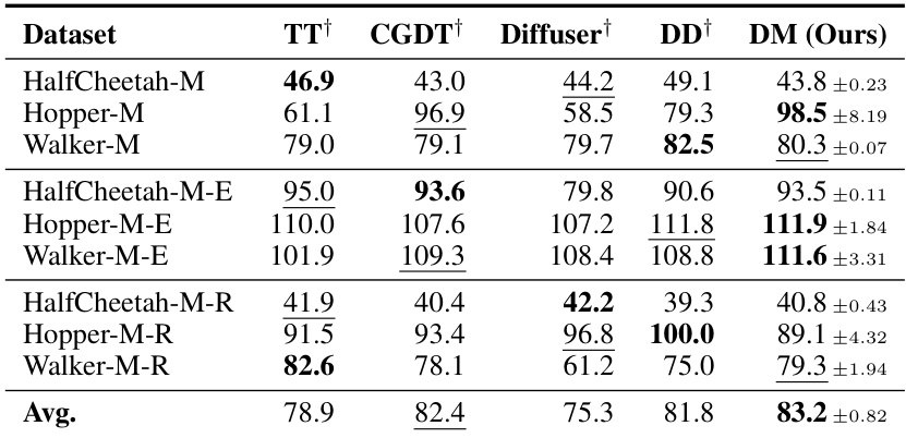
🔼 This table presents the overall performance of the Decision Mamba model and several baseline offline reinforcement learning methods across various datasets. The performance is measured by the normalized score, averaged over four random seeds, with standard deviations reported. The table distinguishes between medium, medium-expert, and medium-replay datasets, reflecting different levels of data quality. Bold and underlined entries highlight the top-performing methods for each dataset.
read the caption
Table 1: Overall Performance. M, M-E, and M-R denotes the medium, medium-expert, and medium-replay, respectively. The results of the baselines marked with † are cited from their original papers. We report the mean and standard deviation of the normalized score with four random seeds. Bold and underline indicate the highest score and second-highest score, respectively.
Full paper#
