↗ OpenReview ↗ NeurIPS Homepage ↗ Chat
TL;DR#
Understanding the complex interplay between extreme weather events and their underlying drivers is crucial for effective climate change mitigation and adaptation strategies. However, existing methods struggle to fully capture the spatio-temporal dynamics of this relationship. The challenge lies in inherent time delays between events and their drivers and the inhomogeneous spatial response of those drivers.
This research tackles this challenge head-on by proposing a novel end-to-end machine learning framework. The framework effectively predicts both extreme events and their drivers jointly from climate data. By quantizing input variables into binary states, the model is trained to recognize only those input features that are strongly correlated with the events. The research demonstrates superior performance on three new synthetic benchmarks and two real-world datasets.
Key Takeaways#
Why does it matter?#
This paper is crucial for climate researchers because it introduces a novel method to identify spatio-temporal drivers of extreme events, a significant challenge in climate data analysis. The synthetic benchmarks and publicly available codebase greatly benefit the community, enabling quantitative evaluations and fostering further research in this critical area. The findings improve understanding of climate change impacts and advance prediction capabilities for extreme weather.
Visual Insights#
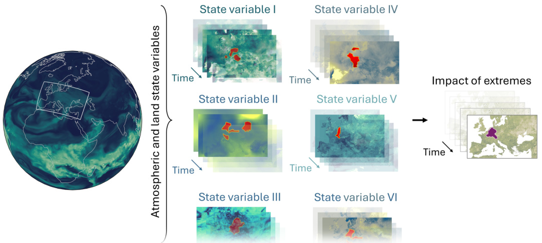
This figure illustrates the core challenge addressed in the paper: identifying the spatio-temporal relationships between extreme events (e.g., agricultural droughts) and their drivers. The challenge stems from the fact that drivers (anomalies in atmospheric and hydrological variables) might occur at different locations and earlier in time than the measurable impact of the extreme event. The figure visually represents this spatio-temporal complexity, showing how drivers from various state variables across different time steps could lead to an extreme event at a later point.
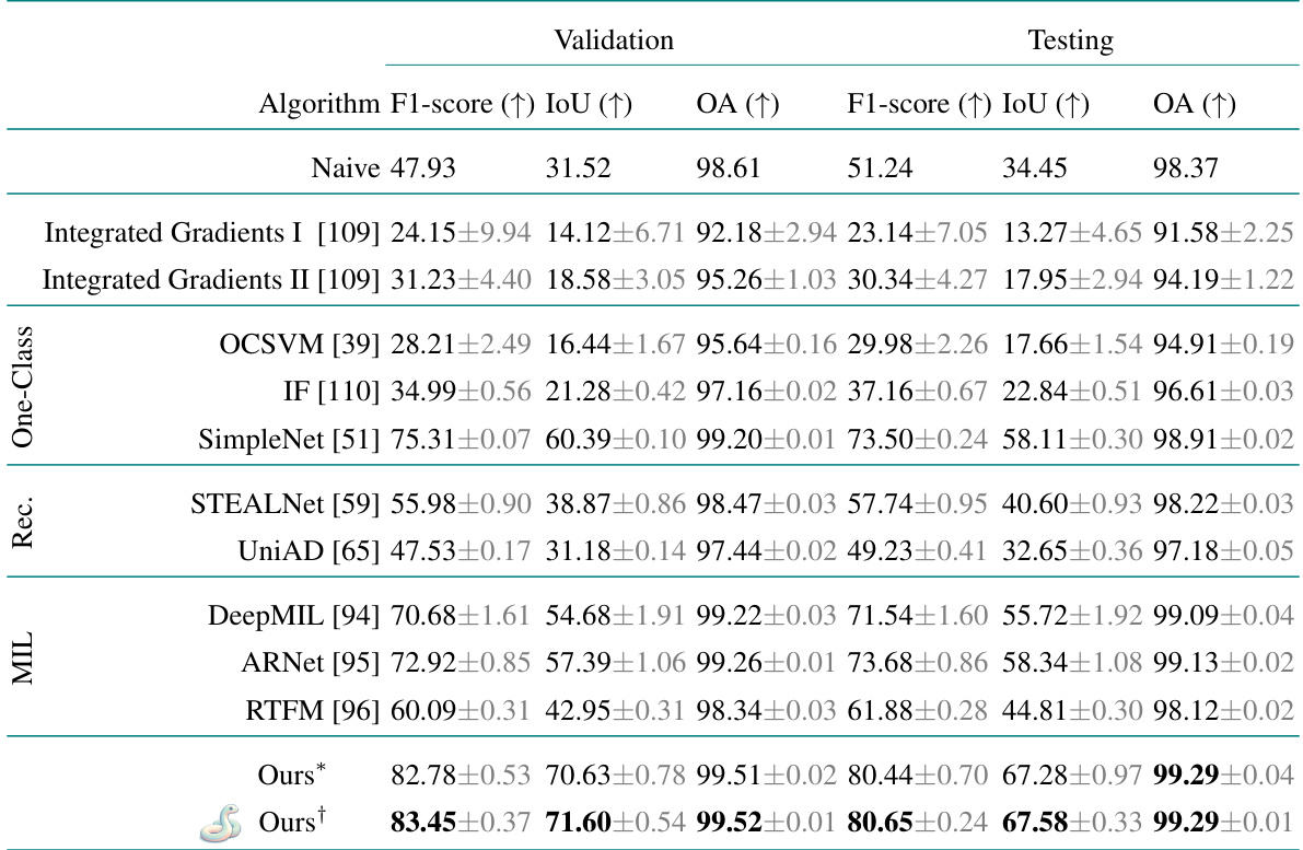
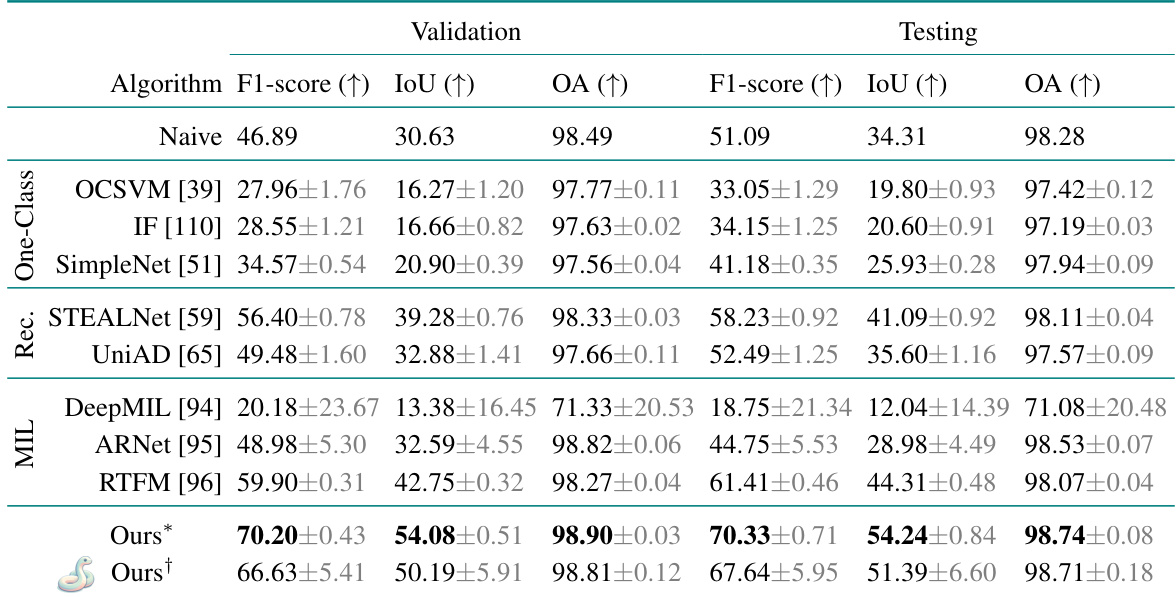
This table presents the quantitative results of the driver detection task on a synthetic dataset based on CERRA reanalysis data. It compares the proposed method’s performance against several baseline approaches, including those based on integrated gradients, one-class unsupervised learning, reconstruction-based methods, and multiple instance learning. The table shows the F1-score, Intersection over Union (IoU), and Overall Accuracy (OA) metrics for both the validation and testing sets, highlighting the best-performing method for each metric.
In-depth insights#
Spatiotemporal Modeling#
Spatiotemporal modeling, in the context of climate research, presents a significant challenge due to the complex interplay of spatial heterogeneity and temporal dynamics. Successfully modeling these interactions is crucial for understanding and predicting extreme events. Key considerations include handling time delays between drivers and events, as well as acknowledging the inhomogeneous spatial response of drivers to extreme phenomena. Advanced machine learning methods, particularly deep learning approaches, are increasingly important for tackling this complex problem, as they offer the ability to learn intricate spatiotemporal relationships from large and complex datasets. However, careful consideration of the model’s limitations such as the assumptions made, the potential for biases in the data, and its generalizability to unseen situations is essential. The creation of reliable and well-defined synthetic datasets is pivotal for quantitative model evaluation, thereby providing a critical foundation for advancement in this research area. Furthermore, the study and consideration of physical consistency within the model’s outputs is important to ensure that findings have scientific validity and that the model is not only statistically accurate but also physically plausible.
Synthetic Data#
The use of synthetic data in this research is a critical methodological innovation addressing the significant challenge of evaluating spatio-temporal driver identification in climate data, where ground truth labels for drivers are scarce. The authors cleverly circumvent this data limitation by designing a framework to generate synthetic data mimicking the properties of real-world climate data, including spatio-temporal correlations and anomalies. This approach allows for robust quantitative evaluation of the proposed model and various baselines and facilitates a nuanced understanding of the model’s strengths and weaknesses in identifying spatio-temporal drivers. The synthetic datasets generated are based on real climate data (CERRA and NOAA) enhancing realism, and incorporate variations in extreme event generation and variable correlation, offering a thorough evaluation setting. The strategy significantly contributes to the advancement of research in this complex domain by providing a reliable and versatile tool for both model development and rigorous assessment.
Anomaly Detection#
Anomaly detection, within the context of climate data analysis, presents a unique challenge. Traditional methods, often relying on pre-defined thresholds or statistical measures, struggle with the inherent complexity and spatio-temporal dynamics of climate data. The difficulty stems from the heterogeneous nature of climate drivers, the non-stationarity of climate signals, and the temporal delays between the occurrences of drivers and their extreme impacts. These challenges highlight the need for advanced techniques capable of learning complex relationships from high-dimensional, noisy data. Machine learning, particularly deep learning, offers a powerful approach to this problem, but even these advanced methods must address challenges such as imbalanced datasets and the lack of clearly labelled anomalous events within climate data. For accurate detection, robust anomaly detection algorithms must also be highly sensitive to spatio-temporal patterns and capable of handling high volumes of multivariate data.
Real-World Results#
A dedicated section on ‘Real-World Results’ would provide critical validation for the proposed spatio-temporal driver identification method. It should present results on multiple, diverse real-world climate datasets, going beyond the synthetic benchmarks. Key aspects to address include the model’s performance (F1-score, IoU, etc.) across different geographic regions and climate types, demonstrating its generalizability. A qualitative analysis of identified drivers, showcasing their spatial and temporal correlation with extreme events, would be crucial, potentially including visualizations. Comparison to relevant existing methods for extreme event prediction or anomaly detection applied to real-world data is essential to highlight the novelty and potential advantages of this approach. Discussion of challenges encountered while applying the method to real-world data (e.g., data quality issues, computational constraints) and insights gained into spatio-temporal relationships between climate variables and extreme events based on real-world findings would enrich the analysis. The section should critically assess how well the synthetic data mimics real-world scenarios and the implications of this for the generalizability of the model. Ultimately, this section is vital to showcase the practical value and robustness of the approach for advancing climate science.
Future Directions#
Future research could explore several promising avenues. Improving the model’s scalability to handle more variables and larger datasets is crucial for real-world applicability. Developing methods for causal inference would strengthen the understanding of driver-extreme relationships beyond correlation. Incorporating more diverse extreme events beyond agricultural droughts would broaden the model’s impact. Investigating the sensitivity of the model to different data resolutions and the impact of various spatio-temporal scales on driver identification warrants further research. Advanced anomaly detection techniques that can handle more complex interactions among variables should be explored. Finally, building a framework to quantitatively assess the accuracy of identified drivers in real-world settings, where the true causal mechanisms remain largely unknown, represents a significant challenge and an important area for future investigation. This could involve developing novel benchmark datasets that are both realistic and interpretable. The insights gained from this research could significantly advance our ability to predict and adapt to the impacts of climate change.
More visual insights#
More on figures

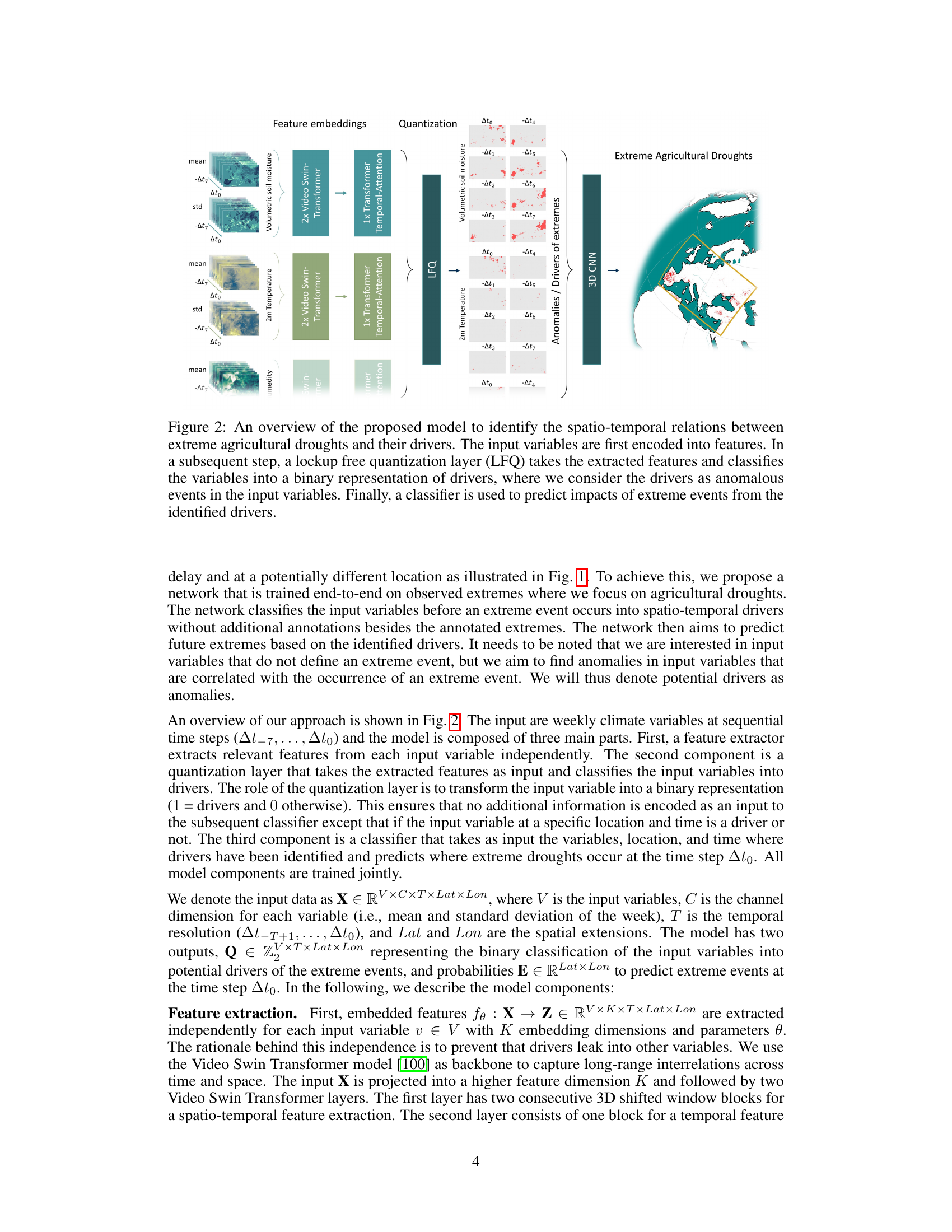
This figure shows the architecture of the proposed model for identifying spatio-temporal relations between extreme agricultural droughts and their drivers. The model consists of three main components: feature extraction, quantization, and classification. The feature extraction component encodes the input variables (e.g., volumetric soil moisture, 2m temperature) into features. The quantization component classifies these features into binary representations of drivers (anomalous events in the input variables). Finally, a classifier predicts impacts of extreme events based on the identified drivers. The model is trained end-to-end on observed extremes (agricultural droughts) to predict future extremes based on the identified drivers.
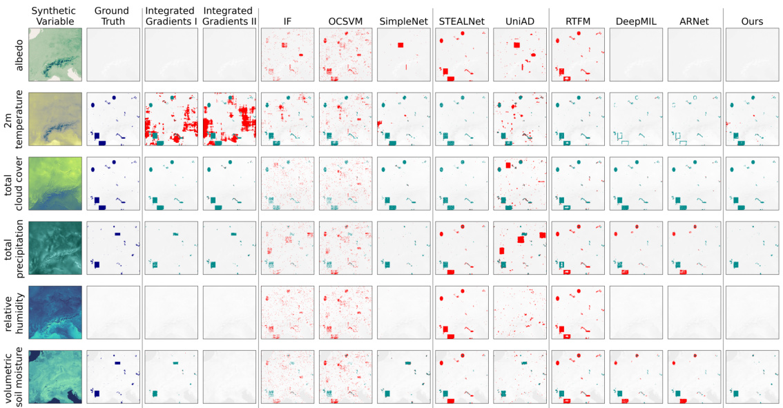
This figure shows a qualitative comparison of different methods for identifying spatio-temporal drivers of extreme events. The top row displays the ground truth (synthetic CERRA reanalysis data) for six variables. Subsequent rows show the predictions of several methods (Integrated Gradients I, Integrated Gradients II, OCSVM, IF, SimpleNet, STEALNet, UniAD, RTFM, DeepMIL, ARNet, and the proposed method), visualizing detected drivers as red pixels and false positives as teal pixels. The results demonstrate the proposed model’s superior performance in accurately identifying spatio-temporal drivers correlated with extreme events (agricultural drought), especially when compared to other baselines which struggle with false positives or fail to capture the spatio-temporal relationships.

This figure shows the F1-score achieved by different anomaly detection methods under varying levels of correlation between input variables and extreme events. The x-axis represents the number of variables correlated with extreme events, ranging from 1/6 to 6/6. The y-axis shows the F1-score. The plot demonstrates how the performance of each method changes as the correlation between variables and extremes increases. This helps to evaluate the robustness and sensitivity of each method to different correlation scenarios. The proposed method (‘Ours’) consistently outperforms the baselines.

This figure illustrates the main goal of the research work presented in the paper. It aims to show the complex spatio-temporal relationships between extreme events (e.g., agricultural droughts) and their potential drivers. The challenge lies in identifying the drivers, which might appear earlier and at different locations compared to the impact of extreme events. The figure visually represents this complexity by showing different state variables (atmospheric and hydrological) over time and space, highlighting the need to identify spatio-temporal anomalies (drivers) that are correlated with the impacts of extreme events.
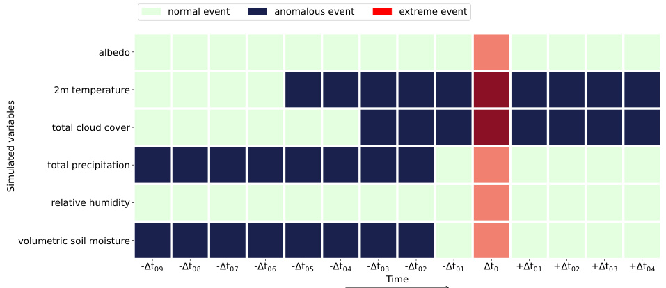
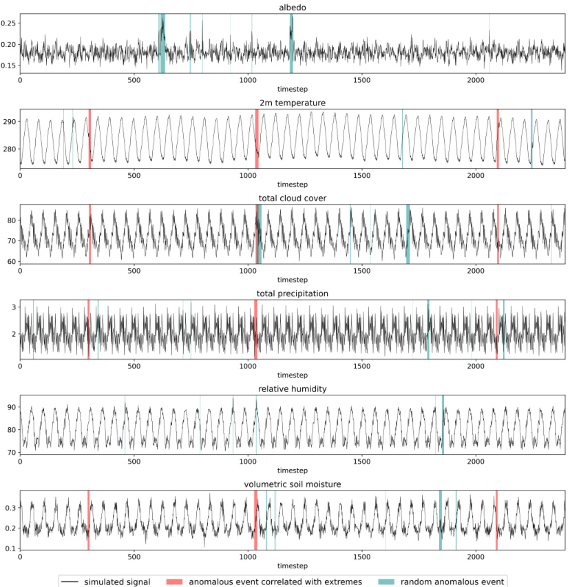
This figure shows a randomly generated coupling matrix used in creating synthetic data for the CERRA dataset. Each row represents a different variable (albedo, 2m temperature, total cloud cover, total precipitation, relative humidity, and volumetric soil moisture). Each column represents a time step relative to an extreme event (indicated as a red block in the figure). The colored blocks within the matrix show the relationship between the variables and extreme events. A dark-colored block indicates an anomalous event in the variable at that time step which is related to the extreme event. The lighter-colored blocks represent either normal events or anomalous events not directly related to the extreme event.

This figure shows examples of the synthetic CERRA reanalysis data generated based on the statistical properties of the real CERRA data. Each subfigure shows a time series of one of six variables, with each column representing a different time step. The data contains both anomalous values and ’normal’ values. The color intensity shows the magnitude of the variable’s values, with brighter colors representing higher values and darker colors representing lower values. Two variables (albedo and relative humidity) are not correlated with the extreme events, while the other four are designed to be correlated to illustrate spatio-temporal relationships between drivers and the extremes.
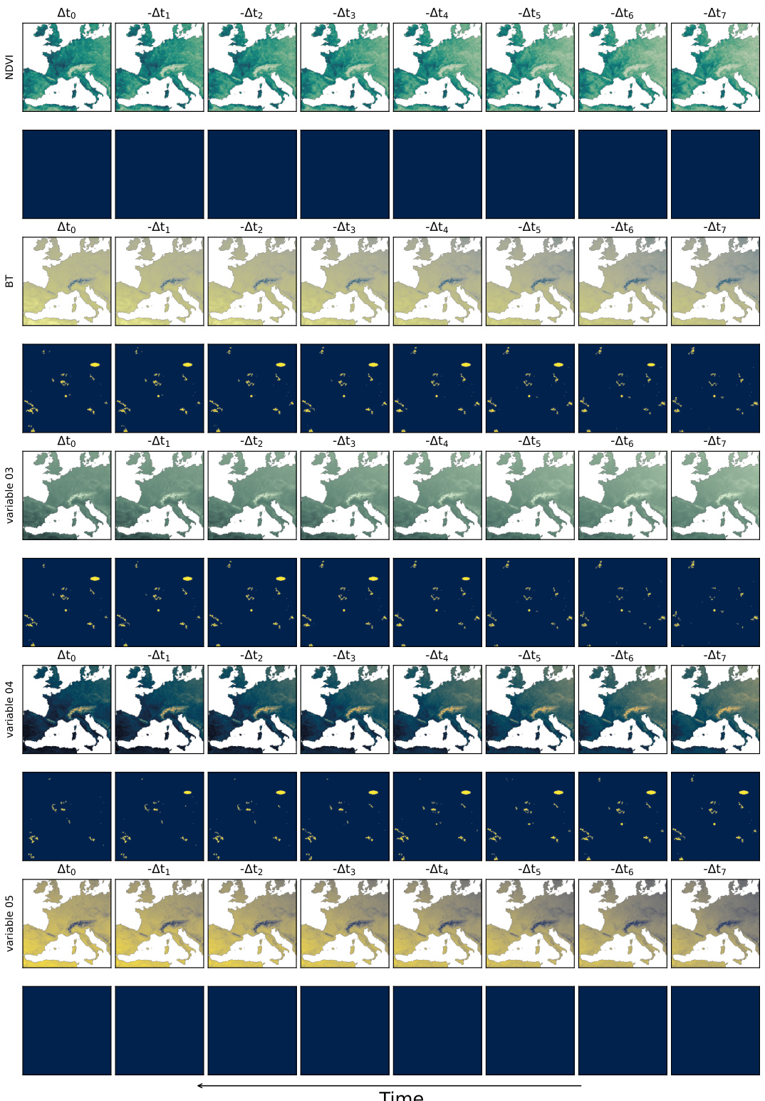
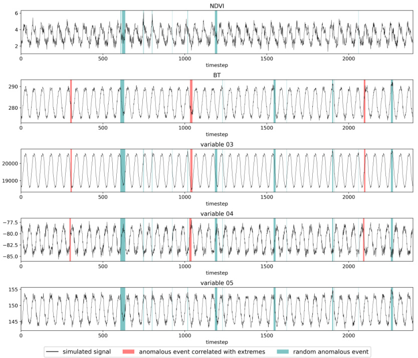
This figure visualizes examples from a synthetic NOAA remote sensing dataset. Each row represents a different variable (NDVI, BT, and three unlabeled variables), showing its values over time. Yellow highlights indicate anomalies or drivers spatio-temporally correlated with extreme events. The caption notes that NDVI and variable 05 are uncorrelated with the extreme events.
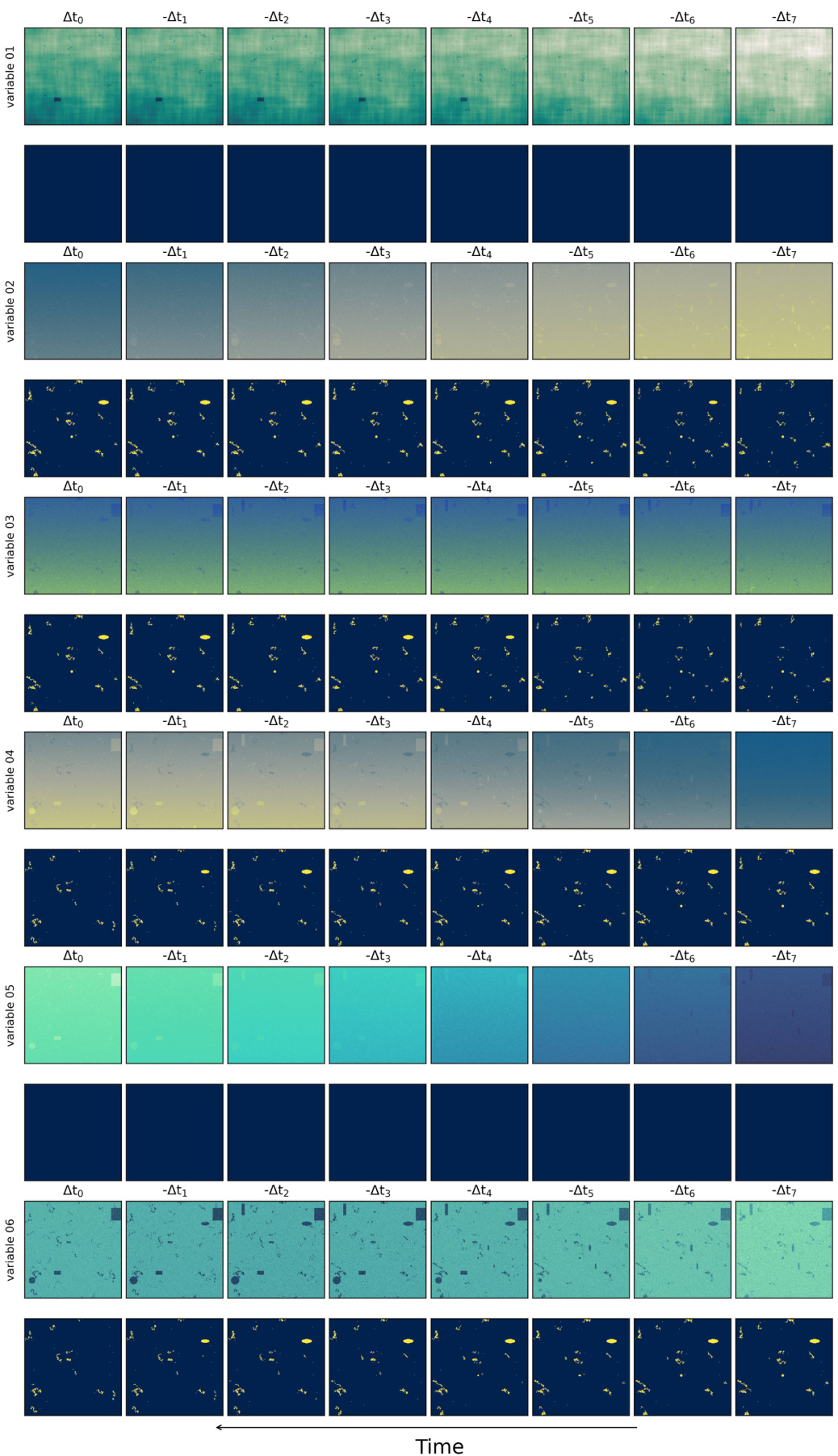
This figure shows examples of the synthetic artificial data generated using the methodology described in Table 5 of the paper. The data includes six variables, each visualized in a separate row. Each row shows a time series (from -Δt7 to Δt0) of the variable’s values in a spatial representation (image). Yellow pixels indicate anomalous events which are considered drivers of extreme events; the absence of yellow indicates no anomalous event. Variables 01 and 05 are specifically indicated as not correlated with the extreme events being modeled.
This figure illustrates the core challenge of the research: identifying the spatio-temporal relationships between extreme weather events (e.g., agricultural droughts, measurable by low vegetation health index) and their drivers. The drivers are defined as anomalies in various land-atmosphere and hydrological state variables (e.g., temperature, soil moisture, evaporation). The difficulty lies in the fact that these drivers can manifest at different locations and earlier in time than the extreme event itself.
This figure illustrates the main challenge addressed in the paper. It shows that the drivers of extreme events (e.g., agricultural droughts) can occur at different locations and earlier in time than the actual extreme events. The goal is to identify the spatio-temporal relations between these drivers and the impacts of extreme events using multivariate climate data.
This figure illustrates the main goal of the research. It highlights the challenge of identifying spatio-temporal relationships between extreme events (e.g., agricultural droughts, measurable by low vegetation health index values) and their drivers. The key difficulty lies in the fact that the drivers (anomalies in atmospheric and hydrological variables) can appear in different locations and at earlier times than the observed impacts of the extreme event. The figure shows schematic representation of this spatio-temporal relationship.
This figure illustrates the core research problem of the paper. The goal is to identify spatio-temporal relationships between measurable impacts of extreme weather events (e.g., agricultural drought measured by vegetation health index, VHI) and their drivers. The challenge lies in the fact that drivers, such as anomalies in atmospheric and hydrological variables, may occur at different locations and earlier in time than the extreme event itself. The figure visually represents this spatio-temporal complexity.

This figure shows the results of ablation studies on the objective functions used in the model. The leftmost panel shows the results when only the loss for drivers L(driver) was used. The next panel shows the result of using only the loss for extreme events L(extreme). The rightmost panel shows the result when both the losses were used. The differences in the results highlight the importance of using both loss functions for better performance.

This figure illustrates the core objective of the research paper: identifying spatio-temporal relations between measurable impacts of extreme events (e.g., agricultural droughts) and their drivers. The challenge is highlighted because the drivers might occur in different locations and/or at earlier times than the extreme event itself.
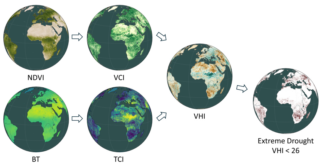
The figure shows how the Vegetation Health Index (VHI) is calculated from two satellite-based products: Normalized Difference Vegetation Index (NDVI) and Brightness Temperature (BT). NDVI measures the greenness of vegetation, while BT measures the surface temperature. Both are combined to create the VHI, which is a measure of vegetation health. Extreme agricultural drought is then defined as VHI values below 26. The figure visually shows the global distribution of NDVI, VCI, TCI, VHI and the resulting extreme drought areas.

This figure displays the spatial distribution of drivers and anomalies related to extreme drought events in Portugal, as identified by the model. The maps show the percentage of weeks with anomalous events for several variables, highlighting areas where the anomalies were most concentrated relative to drought impact.
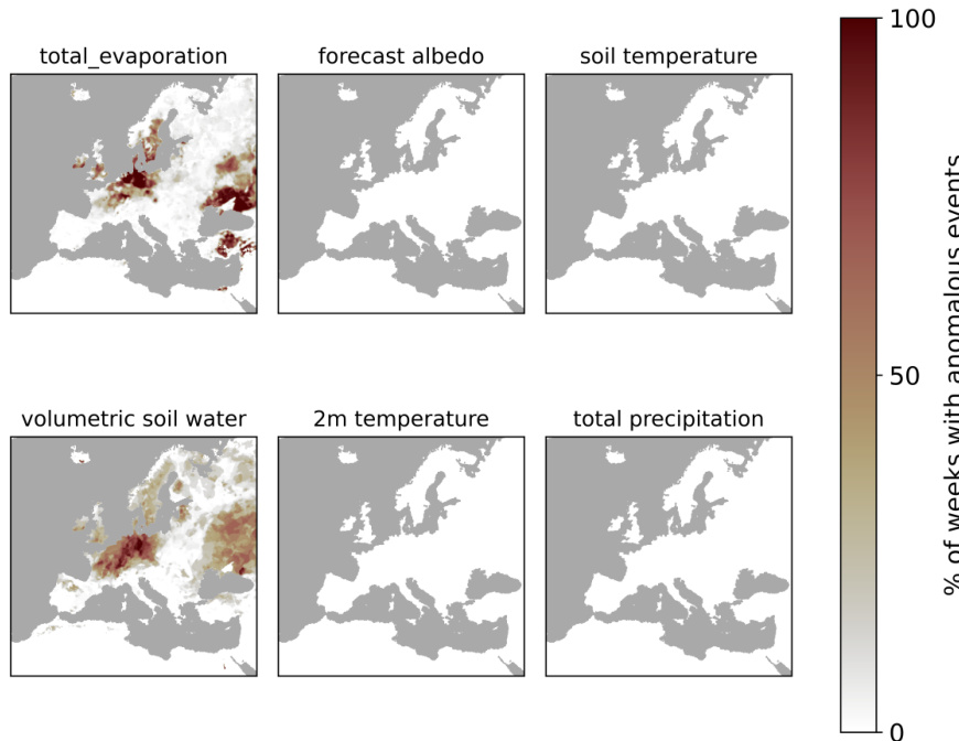
This figure shows the spatial distribution of identified drivers and anomalies related to Portugal, using predictions from the ERA5-Land dataset for the EUR-11 region between 2018 and 2024. Only timeframes with at least 25% of pixels experiencing extreme drought in Portugal were included. The values represent the percentage of weeks with anomalous events, normalized across all such weeks. The spatial concentration of drivers around the regions with extreme drought events demonstrates the model’s ability to identify relevant spatiotemporal patterns.

This figure illustrates the core challenge addressed by the paper. It visually explains the difficulties involved in identifying spatio-temporal drivers of extreme events. These drivers (anomalies in land-atmosphere and hydrological variables) might not occur at the same time or location as the measurable impact of the extreme event (e.g., agricultural drought). The time delay and spatial inhomogeneity create a significant challenge for identifying the causal relationships between drivers and extreme events.
This figure illustrates the main objective of the paper, which is to identify the spatio-temporal relationships between extreme events and their drivers. It highlights the complexity of the task due to the time delays and spatial inhomogeneity of the drivers’ responses. The figure visually shows an extreme event impacting vegetation health and the various potential drivers (anomalies in atmospheric, hydrological, and land state variables) occurring earlier in time and potentially in different locations.

Figure 5(a) shows the spatial distribution of the identified drivers up to 7 weeks before extreme agricultural droughts in Europe. The figure demonstrates the spatial correlation between the predicted drivers and the actual extreme events. Figure 5(b) illustrates the temporal evolution of the drivers and their anomalies leading up to extreme drought events. It showcases the changes in various variables (soil moisture, temperature, etc.) and how their anomalies correlate with the onset of the extreme droughts.

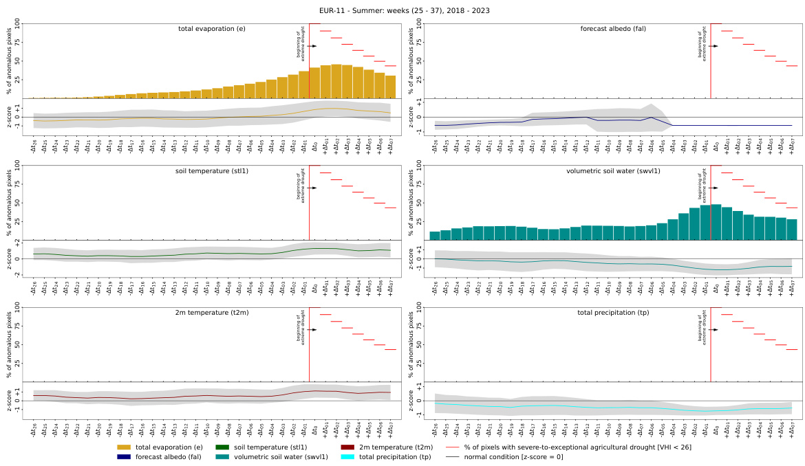
This figure shows the temporal evolution of drivers (anomalies) and their relation to extreme events in the ERA5-Land dataset for Europe. The analysis focuses on pixels experiencing extreme droughts during summer months (weeks 25-38) from 2018 to 2023. The figure visualizes the average distribution of drivers and anomalies over time, highlighting the period leading up to, and following the onset of these extreme events. The red line marks the beginning of the droughts, and the z-score in the bottom graph shows the deviation from the long-term climatological average. This visualization helps to understand the temporal dynamics of drivers and their relationship to extreme events.

This figure illustrates the main goal of the research work presented in the paper. It highlights the challenge of identifying spatio-temporal relationships between extreme events (like agricultural droughts measured by Vegetation Health Index - VHI) and their drivers. The drivers are defined as anomalies in various land-atmosphere and hydrological variables. The difficulty stems from the fact that these drivers might occur at different locations and earlier than the resulting extreme events.

This figure shows the temporal dynamics of the identified drivers and anomalies leading up to extreme drought events in the EUR-11 region of Europe. The analysis focuses on summer months (weeks 25-38) from 2018 to 2023. The plots illustrate the average behavior of key variables (total evaporation, forecast albedo, soil temperature, volumetric soil water, 2m temperature, and total precipitation) in the weeks preceding the drought events. The red vertical lines denote the onset of the droughts, and the shaded area represents the deviation from the climatological mean. The figure provides insights into the temporal relationships between the drivers and the occurrence of extreme droughts.
This figure illustrates the core challenge addressed in the paper: identifying spatio-temporal relationships between extreme events (e.g., agricultural droughts) and their drivers. The key difficulty lies in the temporal lag and spatial heterogeneity between the occurrence of the drivers (anomalies in atmospheric and hydrological variables) and the observable impacts of the extreme events. The figure visually represents this temporal and spatial disconnect, highlighting the challenge of establishing a robust link between these factors.
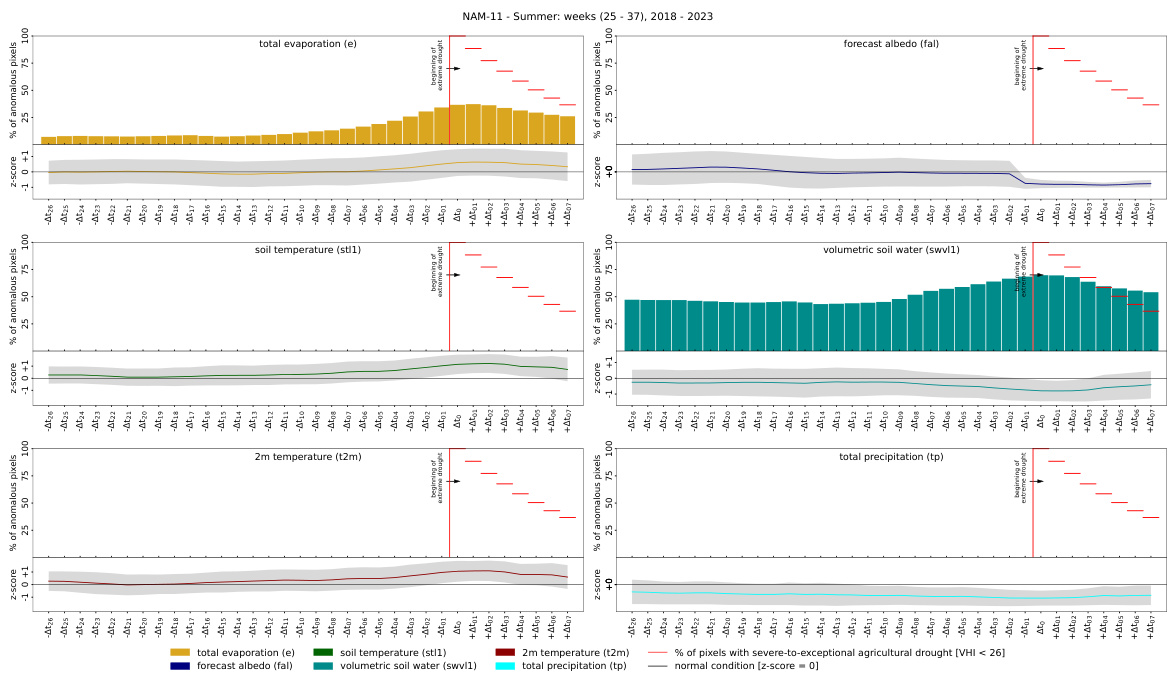
This figure shows the temporal dynamics of identified drivers and anomalies preceding extreme drought events in the EUR-11 region of the ERA5-Land dataset. The analysis focuses on summer months (weeks 25-38) from 2018 to 2023. For each variable (total evaporation, forecast albedo, soil temperature, volumetric soil water, 2m temperature, and total precipitation), it displays the percentage of pixels exhibiting anomalous behavior over time, along with z-scores indicating deviation from the climatological mean. The red line marks the onset of extreme droughts (VHI < 26). The plot helps visualize how different variables change in relation to the onset and progression of the drought.

This figure illustrates the core challenge the paper addresses: identifying spatio-temporal relationships between extreme events (e.g., agricultural droughts, measurable by low vegetation health index values) and their drivers. The key difficulty is that these drivers (anomalies in atmospheric and hydrological variables) may occur at different locations and earlier in time than the observed extreme event. The figure highlights the spatio-temporal aspects of this relationship, making it clear that identifying the connections between them is a complex task.
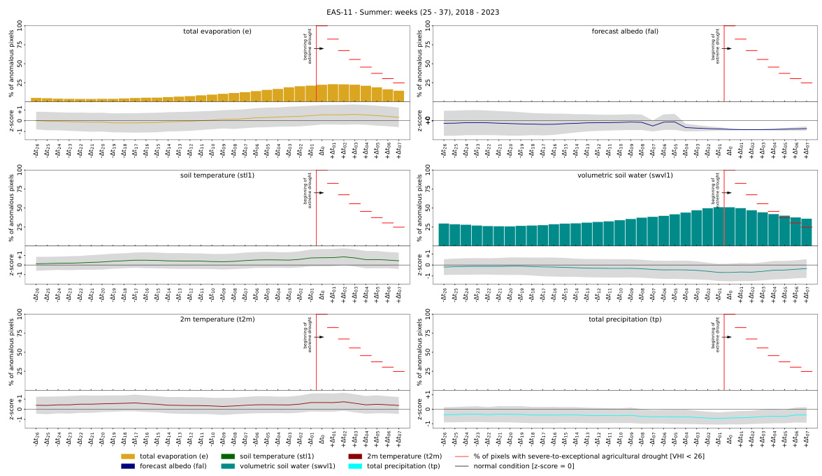
This figure displays the temporal evolution of identified drivers and anomalies in relation to extreme events (agricultural droughts) in the EUR-11 region of ERA5-Land data. The data covers summer weeks (25-38) from 2018 to 2023. For each pixel experiencing an extreme event, the average distribution of driver and anomaly variables across time is calculated and presented. A red line marks the start of extreme droughts (Ato). The z-score shows the deviation from the climatological mean.

The figure provides a detailed overview of the proposed model architecture for identifying spatio-temporal drivers of extreme agricultural droughts. The model consists of three main components: a feature extractor that processes the input climate variables, a quantization layer that converts the features into a binary representation of drivers (anomalies), and a classifier that predicts extreme drought events based on the identified drivers. The model is trained end-to-end to jointly learn the feature representations, driver identification, and drought prediction.

This figure shows the temporal evolution of drivers and anomalies related to extreme events in the ERA5-Land dataset for Europe. It visualizes the average distribution of drivers and anomalies over time for pixels experiencing extreme drought events during summer months (weeks 25-38) between 2018 and 2023. The red line marks the onset of extreme droughts. The Z-score in the lower graphs indicates how much the values deviate from the average.

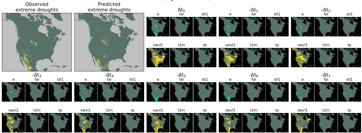
This figure shows the qualitative results of the proposed model on ERA5-Land data for the EUR-11 region. It displays the identified drivers and anomalies for each variable, along with the model’s prediction of extreme agricultural droughts. The top-left shows the observed and predicted extreme droughts, and subsequent columns show identified driver anomalies for various atmospheric and land state variables including forecast albedo (fal), soil temperature (stl1), total evaporation (e), total precipitation (tp), volumetric soil water (swvl1), and 2m temperature (t2m) up to 7 weeks before the extreme event (t=0).
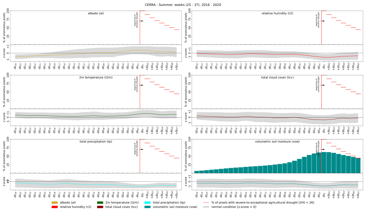
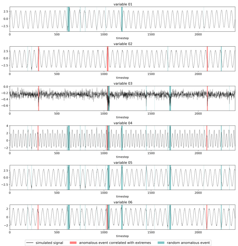
The figure visualizes the generated synthetic signals for six different variables from the synthetic CERRA reanalysis dataset. Each variable’s time series is shown for a specific location (latitude 50, longitude 50). The signals consist of three components: normal base signals, anomalies correlated with extreme events, and random anomalies. The anomalies correlated with extremes are designed to mimic real-world drivers of extreme events, while the random anomalies represent background noise or unrelated variations.
More on tables

This table presents a comparison of different algorithms for driver detection on a synthetic CERRA reanalysis dataset. It shows the F1-score, Intersection over Union (IoU), and Overall Accuracy (OA) for both validation and testing sets. The algorithms compared include several anomaly detection methods (one-class, reconstruction-based, multiple instance learning), interpretable forecasting methods, and the authors’ proposed method. The best-performing algorithm in each metric is highlighted.

This table presents the quantitative results of the driver detection task on a synthetic dataset based on CERRA reanalysis. It compares the proposed method’s performance against several baselines, including methods from interpretable forecasting, one-class unsupervised, reconstruction-based, and multiple instance learning approaches. The results are evaluated using three metrics: F1-score, Intersection over Union (IoU), and Overall Accuracy (OA). For each metric, the best performing algorithm is highlighted in bold. The standard deviation is reported to reflect the variability of the results across three runs.
This table presents the quantitative results of driver detection experiments performed on a synthetic dataset generated using CERRA reanalysis data. It compares the proposed method with several baseline methods across different metrics: F1-score (higher is better, indicates the balance between precision and recall), IoU (Intersection over Union, higher is better, indicates the overlap between predicted and ground truth driver locations), and OA (Overall Accuracy, higher is better, indicates the percentage of correctly classified pixels). The best performance for each metric is highlighted in bold, and standard deviations over 3 independent runs are provided.

This table presents the quantitative results of the driver detection task on a synthetic dataset based on the CERRA reanalysis. It compares the proposed method’s performance against several baseline approaches, including those based on interpretable forecasting, one-class, reconstruction-based, and multiple instance learning methods. The table shows the F1-score, Intersection over Union (IoU), and Overall Accuracy (OA) metrics for both validation and test sets. The best performance for each metric is highlighted in bold, and standard deviations across three runs are also included.
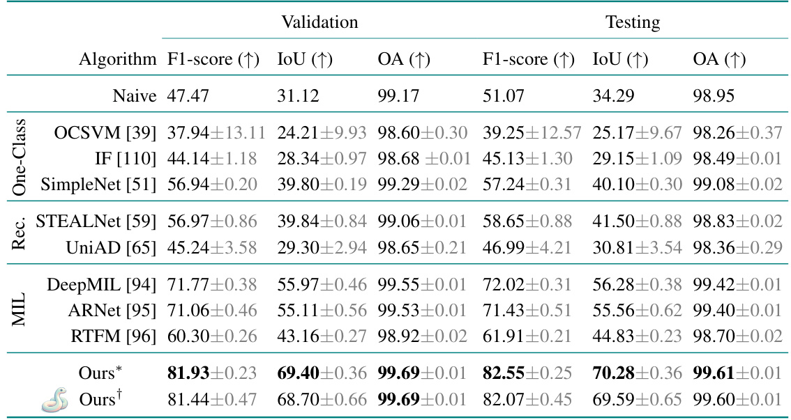
This table presents the quantitative results of the driver detection task on the synthetic CERRA dataset. It compares the performance of the proposed model against several baselines, including those based on interpretable forecasting, one-class unsupervised methods, reconstruction-based methods, and multiple instance learning. The table displays F1-score, Intersection over Union (IoU), and Overall Accuracy (OA) metrics for both validation and test sets, highlighting the best performance for each metric.
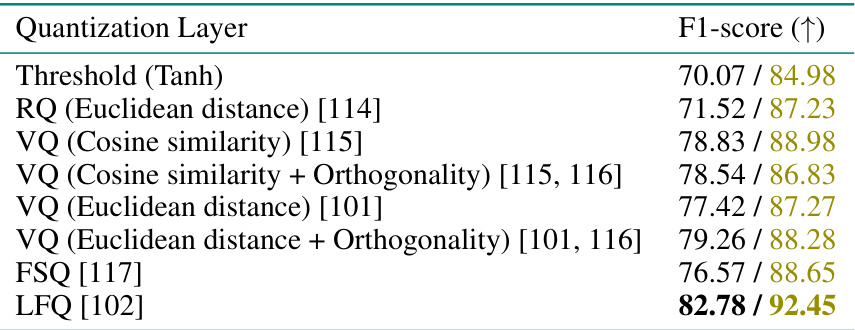
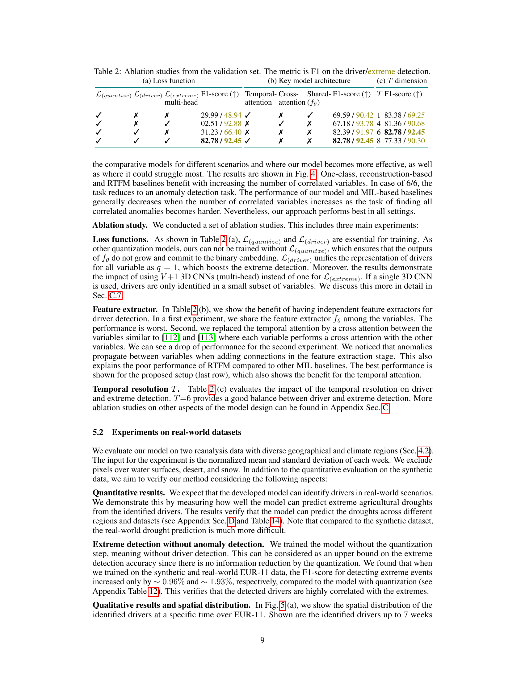
This table presents the results of ablation studies conducted on the quantization layer of the proposed model. Different quantization methods were tested: Threshold (Tanh), Random Quantization (RQ), Vector Quantization (VQ) with and without orthogonality, Finite Scalar Quantization (FSQ), and Lookup-free Quantization (LFQ). The F1-score, a metric evaluating the balance between precision and recall, is reported for both driver and extreme event detection for each method. The table shows how the choice of quantization method significantly impacts the model’s performance.
This table presents the ablation study on different quantization methods used in the proposed model for identifying spatio-temporal drivers of extreme events. The F1-score metric evaluates the performance of each quantization method on both driver and extreme event detection tasks. The results show that the Lockup-free quantization (LFQ) method outperforms other methods.

This table presents the quantitative results of the driver detection task on a synthetic dataset based on CERRA reanalysis data. It compares the proposed method’s performance against several baseline methods across three evaluation metrics: F1-score, Intersection over Union (IoU), and Overall Accuracy (OA). The results are shown for both the validation and test sets, with the best performance for each metric highlighted. The standard deviation for three independent runs is also included, providing insights into the reliability of the results.
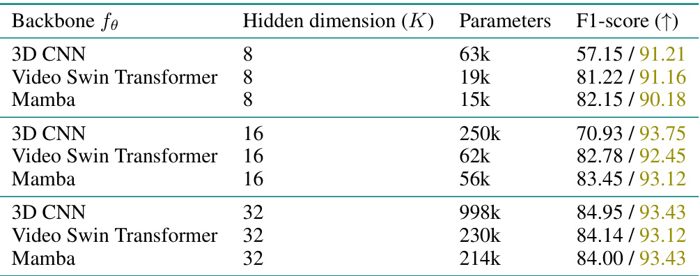
This table presents the ablation study on the backbone used for feature extraction in the proposed model. Three different backbones are compared: 3D CNN, Video Swin Transformer, and Mamba. For each backbone, three different hidden dimensions (K) are tested: 8, 16, and 32. The table shows the number of parameters for each configuration and the resulting F1-score on both driver and extreme detection tasks. This helps to understand the impact of backbone architecture and its complexity on the performance of the model.

This table presents the quantitative results of the driver detection task on a synthetic dataset based on CERRA reanalysis data. It compares the proposed approach against several baseline methods, including those based on interpretable forecasting, one-class unsupervised learning, reconstruction-based methods, and multiple instance learning. The table provides the F1-score, Intersection over Union (IoU), and Overall Accuracy (OA) metrics for both validation and test sets, highlighting the best-performing model for each metric.

This table presents the quantitative results of the driver detection task on a synthetic dataset based on CERRA reanalysis data. It compares the proposed model’s performance to several baseline methods across three evaluation metrics: F1-score, Intersection over Union (IoU), and Overall Accuracy (OA). The results are shown for both the validation and test sets. The best performing model for each metric on each set is highlighted in bold. The ± symbol indicates the standard deviation calculated across three separate runs for each model, providing an estimate of the variability in performance.

This table presents a quantitative comparison of the proposed driver detection model against several baseline methods on a synthetic dataset mimicking CERRA reanalysis data. The performance is evaluated across three metrics: F1-score, Intersection over Union (IoU), and Overall Accuracy (OA). The results are shown for both validation and testing sets, and the best performance for each metric is highlighted.

This table presents the quantitative results of the driver detection task on the synthetic CERRA dataset. It compares the proposed model’s performance against several baseline methods across three evaluation metrics: F1-score, Intersection over Union (IoU), and Overall Accuracy (OA). The results are shown for both the validation and test sets, allowing for an assessment of the model’s generalization capabilities. The best performance for each metric is highlighted in bold. Standard deviation values are included to indicate the variability of the results across three independent experimental runs. The naive baseline provides a simple comparison, showing results when all variables are assumed to be drivers for all extreme event pixels.

This table shows the impact of different thresholds for defining extreme drought events (using the Vegetation Health Index, VHI) on the model’s ability to detect them. It compares the F1-score of the model for three different VHI thresholds (VHI<26, VHI<40, VHI<50) when using either only soil temperature (stl1) or a set of multiple input variables ({t2m, fal, e, tp, stl1, swvll}) for prediction. The results illustrate the sensitivity of extreme event detection to how extreme events are defined.

This table presents the quantitative results of the driver detection task on the synthetic CERRA dataset. It compares the proposed method’s performance against several baseline methods across three evaluation metrics: F1-score, Intersection over Union (IoU), and Overall Accuracy (OA). The best result for each metric is highlighted in bold. Standard deviations across three separate runs are also provided, giving a measure of the model’s consistency. The table shows the performance on both the validation and test splits of the dataset, giving a comprehensive evaluation of the different models’ performance.
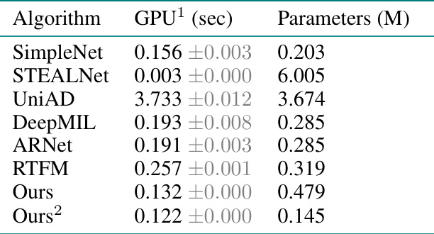
This table presents the quantitative results of the driver detection task on a synthetic dataset based on CERRA reanalysis. It compares the proposed model’s performance against several baseline methods across different metrics: F1-score, IoU, and overall accuracy (OA). The best performing model for each metric is highlighted in bold. The standard deviation across three runs is included to show the consistency of the results.

This table presents the quantitative results of the driver detection task on the synthetic CERRA dataset. It compares the proposed model’s performance against several baseline methods across various metrics: F1-score, Intersection over Union (IoU), and Overall Accuracy (OA). The results are shown for both validation and test sets, and standard deviations are provided to indicate the stability of the results. The best performance for each metric is clearly highlighted.

This table presents the quantitative results of driver detection experiments conducted on a synthetic CERRA reanalysis dataset. It compares the proposed method’s performance (F1-score, IoU, and overall accuracy) against several baseline methods representing various anomaly detection approaches (one-class, reconstruction-based, and multiple instance learning), as well as a naive baseline. The table highlights the best performing model for each evaluation metric, showing the superiority of the proposed approach. The standard deviation for three experimental runs is included to demonstrate reliability.

This table presents a quantitative comparison of the proposed driver detection method against several baseline methods on a synthetic CERRA reanalysis dataset. The metrics used for comparison include F1-score, Intersection over Union (IoU), and Overall Accuracy (OA). The best-performing method for each metric is highlighted in bold. The standard deviation across three runs is also provided to show the variability of the results.
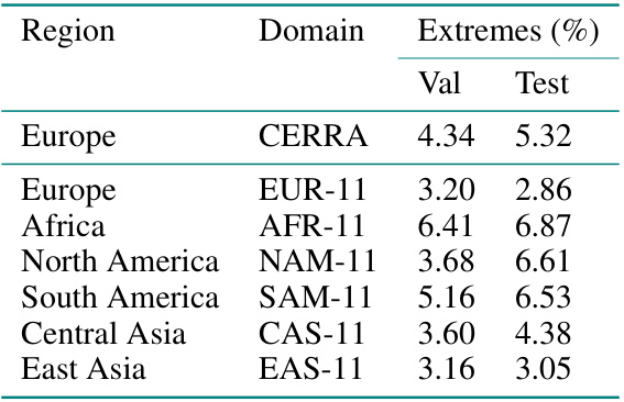
This table presents the quantitative results of driver detection experiments conducted on a synthetic dataset based on the CERRA reanalysis. It compares the performance of the proposed model against several baseline methods across different evaluation metrics: F1-score (higher is better, indicating accuracy in identifying drivers), IoU (Intersection over Union, higher is better, measuring the overlap between predicted and actual driver regions), and OA (Overall Accuracy, higher is better, showing the overall correctness of the prediction). The best performance in each metric for each baseline is highlighted. The standard deviations across three separate runs are provided, illustrating the stability and reliability of the results. The ‘Naive’ baseline represents a simple strategy for comparison.
Full paper#
