TL;DR#
Graph Neural Networks (GNNs) are powerful but struggle to consistently capture relationships between graphs across layers. This often leads to inconsistent similarity rankings and reduced classification accuracy, especially when compared to more stable graph kernel methods that rely on pre-defined kernels. These kernels, while effective, suffer from a lack of non-linearity and computational limitations for large datasets.
This paper addresses these limitations by introducing a novel consistency loss function. The function enforces the similarity of graph representations to remain consistent across different layers, drawing inspiration from the Weisfeiler-Lehman optimal assignment (WLOA) kernel. The results demonstrated significant improvements in graph classification accuracy across various GNN backbones and datasets, validating the hypothesis that consistent similarity preservation across layers is crucial for accurate graph representation.
Key Takeaways#
Why does it matter?#
This paper is crucial because it bridges the gap between neural network methods and kernel approaches in graph representation learning. It introduces a novel consistency loss function to improve GNNs’ ability to capture relational structures consistently across layers, impacting graph classification accuracy. This work offers a new perspective on graph representation learning and opens avenues for further research into improving the consistency and effectiveness of GNNs.
Visual Insights#
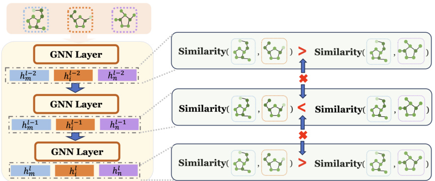
🔼 This figure demonstrates the inconsistency in similarity relationships captured by graph neural networks (GNNs) across different layers. Cosine similarity is calculated between three molecules from the NCI1 dataset using graph representations obtained from three consecutive GIN layers (layer 0, 1 and 2). The figure shows that the relative similarity between the molecules changes across layers. For example, two molecules that are very similar at layer 0 might show reduced similarity at layer 1, and then increased similarity again at layer 2. This inconsistency in similarity relationships highlights a limitation of common GNNs in preserving relational structures during the message-passing process.
read the caption
Figure 1: Cosine similarity of three molecules from the NCI1 dataset, evaluated using graph representations from three consecutive GIN layers. Common GNN models fail to preserve relational structures across the layers.

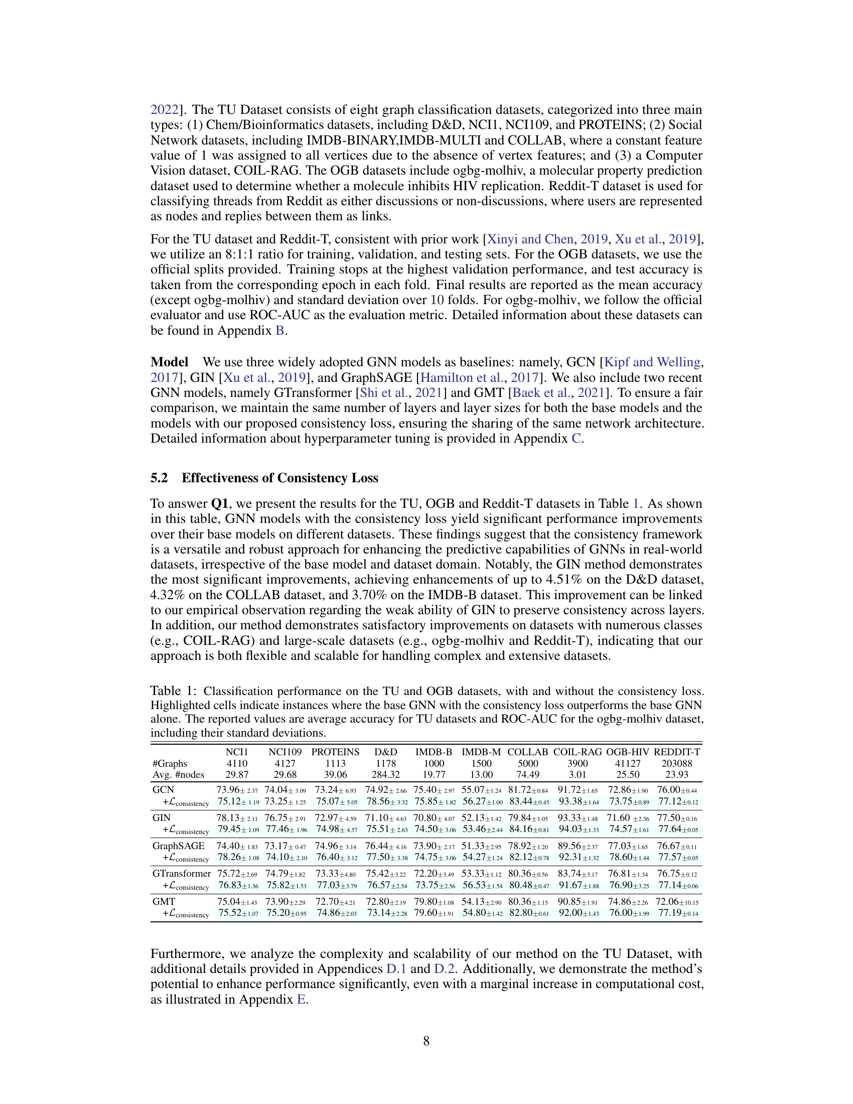
🔼 This table presents the classification performance of several Graph Neural Networks (GNNs) on various graph datasets, both with and without the proposed consistency loss. It shows the average accuracy (for TU datasets) or ROC-AUC score (for OGB-HIV) for each model and dataset. Highlighted entries indicate cases where adding the consistency loss improved performance. The table helps demonstrate the effectiveness of the consistency loss across multiple GNN architectures and diverse datasets.
read the caption
Table 1: Classification performance on the TU and OGB datasets, with and without the consistency loss. Highlighted cells indicate instances where the base GNN with the consistency loss outperforms the base GNN alone. The reported values are average accuracy for TU datasets and ROC-AUC for the ogbg-molhiv dataset, including their standard deviations.
In-depth insights#
Graph Rep Consistency#
The concept of ‘Graph Rep Consistency’ centers on the reliable preservation of similarity relationships between graphs across different layers or iterations of a graph representation learning model. Inconsistency in these relationships, a known issue in many Graph Neural Networks (GNNs), undermines the model’s ability to accurately capture structural information. The research likely explores methods to enforce this consistency, perhaps by modifying loss functions, or introducing constraints into the model’s architecture. A key aspect is likely the comparison of GNNs with graph kernel methods (like Weisfeiler-Lehman subtree kernels), which often exhibit more consistent similarity capture due to their reliance on predefined, iterative similarity measures. The core of this work might involve proposing a novel framework or a loss function to address this inconsistency and improve overall model performance on graph classification or other graph-related tasks, while providing a theoretical justification for its effectiveness. This would bridge the gap between the consistency often seen in graph kernels and the variability found in learned representations of GNNs.
Iterative Graph Kernels#
The concept of “Iterative Graph Kernels” introduces a novel perspective on graph representation learning. It elegantly bridges the gap between traditional graph kernel methods and the more modern Graph Neural Networks (GNNs). The core idea revolves around iteratively refining graph representations, analogous to the message-passing mechanism in GNNs. This iterative process allows for the progressive capture of increasingly complex structural information within the graph. By defining iterative graph kernels (IGKs) formally, the authors lay the groundwork for exploring crucial properties like monotonic decrease and order consistency. These properties ensure that similar graphs remain similar across iterations and that the relative similarity rankings are consistently maintained, which enhances the overall classification performance. The study’s analysis of WL-subtree and WLOA kernels highlights the significance of these consistency properties, explaining why WLOA generally outperforms WL-subtree. This framework provides valuable insights into designing more effective graph kernels and potentially informs the design of more robust and consistent GNN architectures.
Consistency Loss#
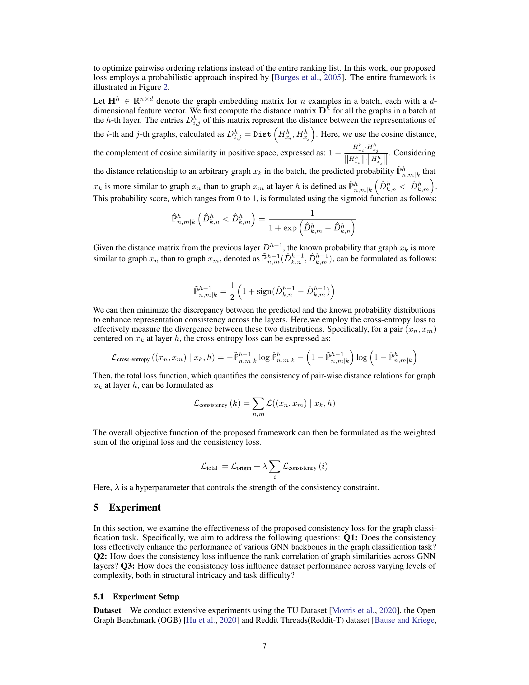
The proposed ‘Consistency Loss’ aims to improve graph classification by enforcing consistent similarity relationships between graph representations across different layers of a Graph Neural Network (GNN). This addresses a key limitation of GNNs, which often fail to maintain consistent similarities across layers, hindering performance. The loss function is designed to align the ranking of graph similarities across layers, ensuring that similar graphs remain similar throughout the network’s processing. This approach is inspired by the analysis of Weisfeiler-Lehman (WL) graph kernels, particularly the WLOA kernel, which exhibits asymptotic consistency in similarity rankings across iterations. By applying this principle to GNNs, the consistency loss encourages the GNN to learn representations that better capture relational structures in the data, leading to improved classification accuracy. The loss is model-agnostic, meaning it can be applied to various GNN architectures without modification. Empirical results demonstrate significant performance gains across multiple datasets and GNN backbones, supporting the effectiveness of this novel loss function in enhancing graph representation learning and classification.
Empirical Analysis#
An empirical analysis section in a research paper would typically present the results of experiments designed to test the hypotheses or claims made earlier in the paper. A thoughtful analysis would go beyond simply reporting metrics; it would discuss the implications of the findings. For example, it would explore whether the results support the hypotheses, showing a clear connection between the experimental design and the conclusions drawn. It would also address any unexpected findings, potential limitations of the experimental methodology, or the generalizability of the results to other settings. A strong empirical analysis will carefully consider and address potential confounding factors or biases, demonstrating a rigorous and nuanced understanding of the data. Furthermore, it should present the results in a clear and accessible manner, using appropriate visualizations (e.g., graphs, tables) to highlight key findings and trends. A good analysis may also include comparisons with existing work or benchmarks, placing the findings in the broader context of the field. Robust error analysis is crucial, ensuring that the observed effects are statistically significant and not due to random variation. Finally, the discussion should connect the empirical findings back to the paper’s overall aims and contributions, explaining how the results contribute to the knowledge in the area.
Future Directions#
Future research could explore extending consistency-driven methods beyond graph classification to other graph-related tasks like graph generation and regression. Investigating the interplay between consistency and other crucial aspects of GNNs, such as explainability and robustness, is warranted. A deeper theoretical understanding of the consistency principle, possibly involving information theory or graph theory, would strengthen the foundations of this approach. Furthermore, developing more efficient algorithms for enforcing consistency, perhaps through approximation techniques or specialized hardware, is crucial for scalability to massive datasets. Finally, exploring applications in domains where relational structures are critical, like drug discovery or materials science, would demonstrate the practical impact of this method and could lead to novel insights.
More visual insights#
More on figures

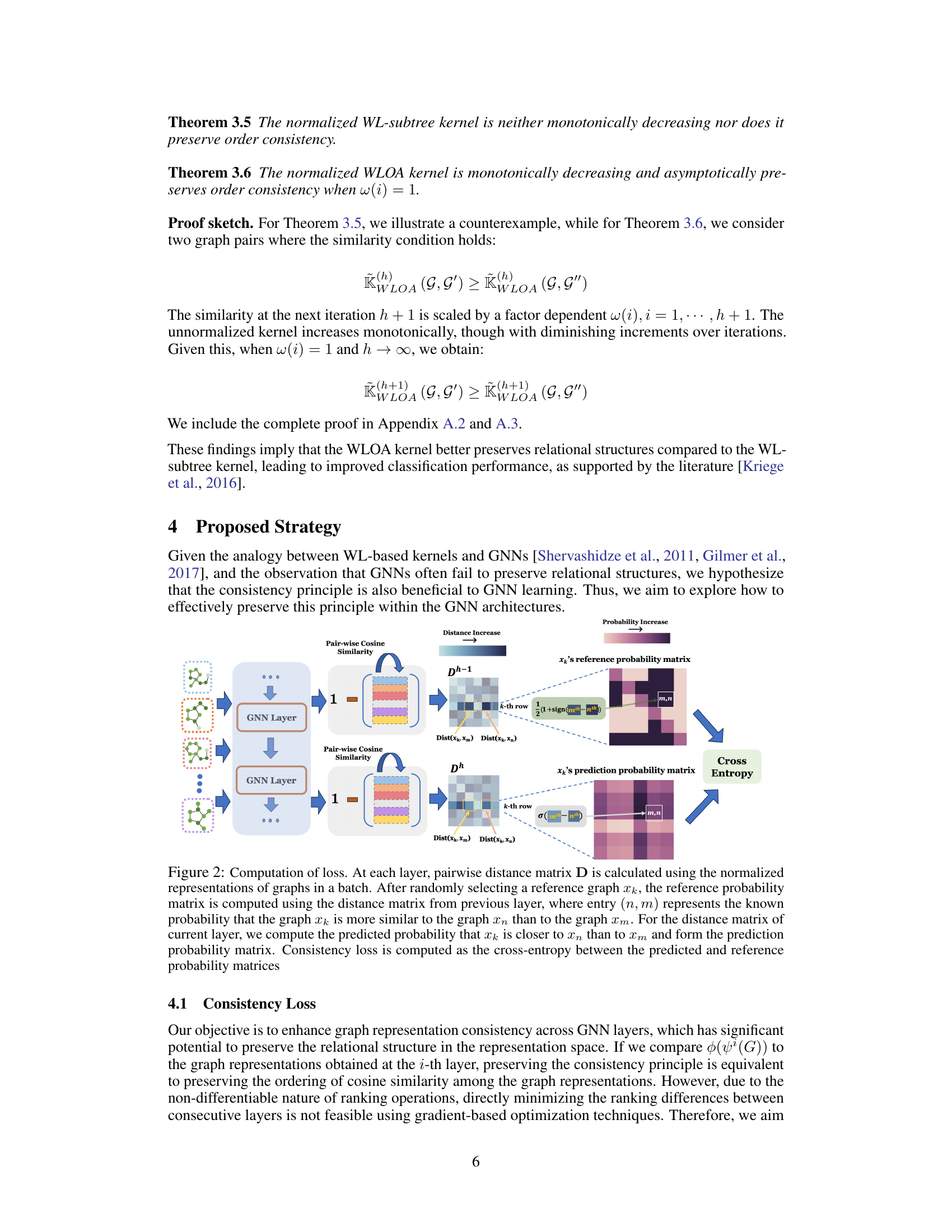
🔼 This figure illustrates the computation of the consistency loss, which is designed to align the ranking of graph similarities across GNN layers. The process involves calculating pairwise distance matrices (D) at each layer using graph representations. A reference graph is randomly selected, and a reference probability matrix is created based on distances from the previous layer. A prediction probability matrix is then generated using the current layer’s distances. The consistency loss is finally computed as the cross-entropy between the reference and prediction matrices.
read the caption
Figure 2: Computation of loss. At each layer, pairwise distance matrix D is calculated using the normalized representations of graphs in a batch. After randomly selecting a reference graph xk, the reference probability matrix is computed using the distance matrix from previous layer, where entry (n, m) represents the known probability that the graph xk is more similar to the graph xn than to the graph xm. For the distance matrix of current layer, we compute the predicted probability that xk is closer to xn than to xm and form the prediction probability matrix. Consistency loss is computed as the cross-entropy between the predicted and reference probability matrices.

🔼 This figure illustrates the computation of the consistency loss, a key component of the proposed method in the paper. It shows how pairwise distances between graph representations are used to generate probability matrices at each layer. These matrices quantify the similarity relationships between graphs, and the consistency loss measures the discrepancy between these relationships across consecutive layers. This helps to ensure consistent similarity rankings across layers during training.
read the caption
Figure 2: Computation of loss. At each layer, pairwise distance matrix D is calculated using the normalized representations of graphs in a batch. After randomly selecting a reference graph xk, the reference probability matrix is computed using the distance matrix from previous layer, where entry (n, m) represents the known probability that the graph xk is more similar to the graph xn than to the graph xm. For the distance matrix of current layer, we compute the predicted probability that xk is closer to xn than to xm and form the prediction probability matrix. Consistency loss is computed as the cross-entropy between the predicted and reference probability matrices.
More on tables
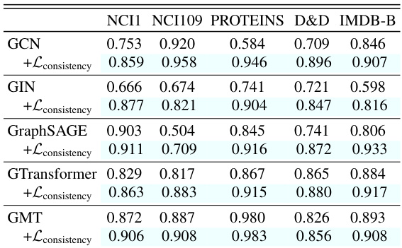
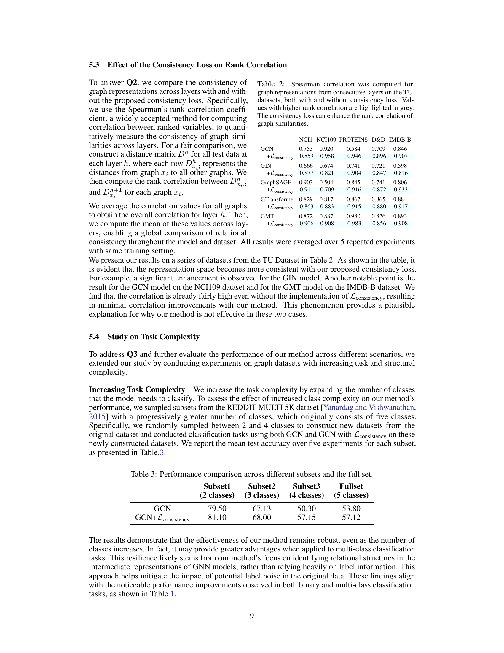
🔼 This table presents the Spearman rank correlation coefficients, measuring the consistency of graph similarity rankings across consecutive layers of various GNN models. It compares the results with and without the proposed consistency loss applied to the models. Higher correlation values indicate stronger consistency in the similarity rankings between layers. The results are shown for several graph datasets from the TU benchmark dataset.
read the caption
Table 2: Spearman correlation was computed for graph representations from consecutive layers on the TU datasets, both with and without consistency loss. Values with higher rank correlation are highlighted in grey. The consistency loss can enhance the rank correlation of graph similarities.

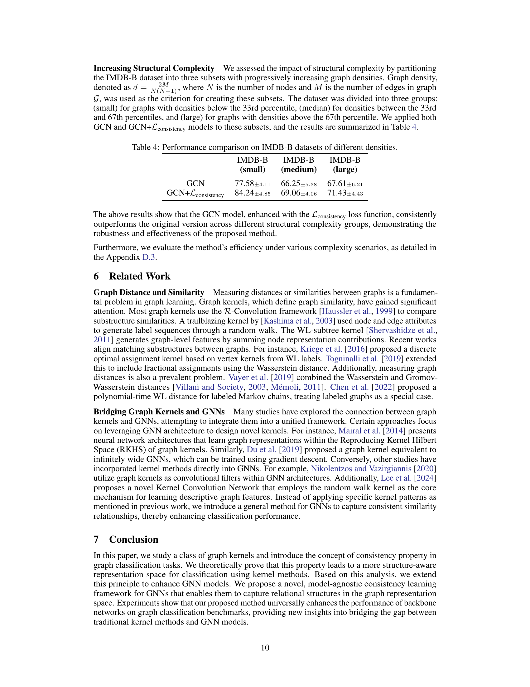
🔼 This table presents the performance comparison of GCN and GCN enhanced with consistency loss across different subsets of Reddit dataset with varying number of classes (2,3,4,5). The subsets are created by randomly sampling classes from the original dataset. The table shows the mean accuracy over five experiments for each subset.
read the caption
Table 3: Performance comparison across different subsets and the full set.

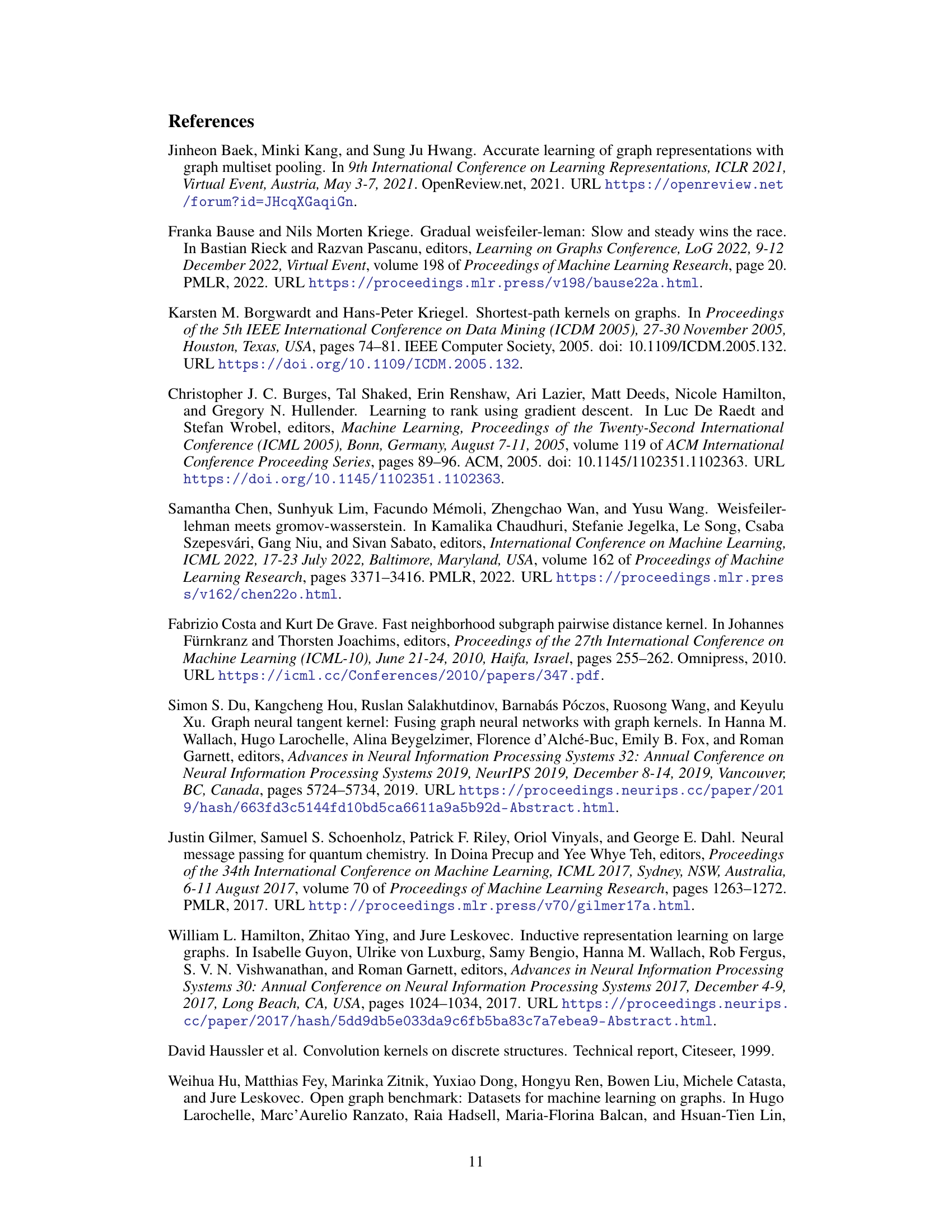
🔼 This table presents the classification performance comparison between the GCN model and the GCN model enhanced with the proposed consistency loss (GCN+Lconsistency). The comparison is conducted on three subsets of the IMDB-B dataset, categorized based on their graph density: (small), (medium), and (large). The results demonstrate the effectiveness of the consistency loss in improving classification performance across different levels of graph structural complexity.
read the caption
Table 4: Performance comparison on IMDB-B datasets of different densities.
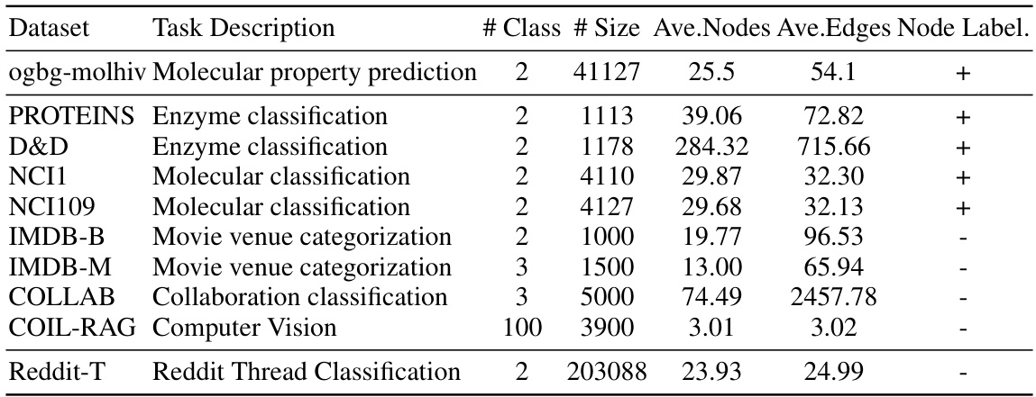
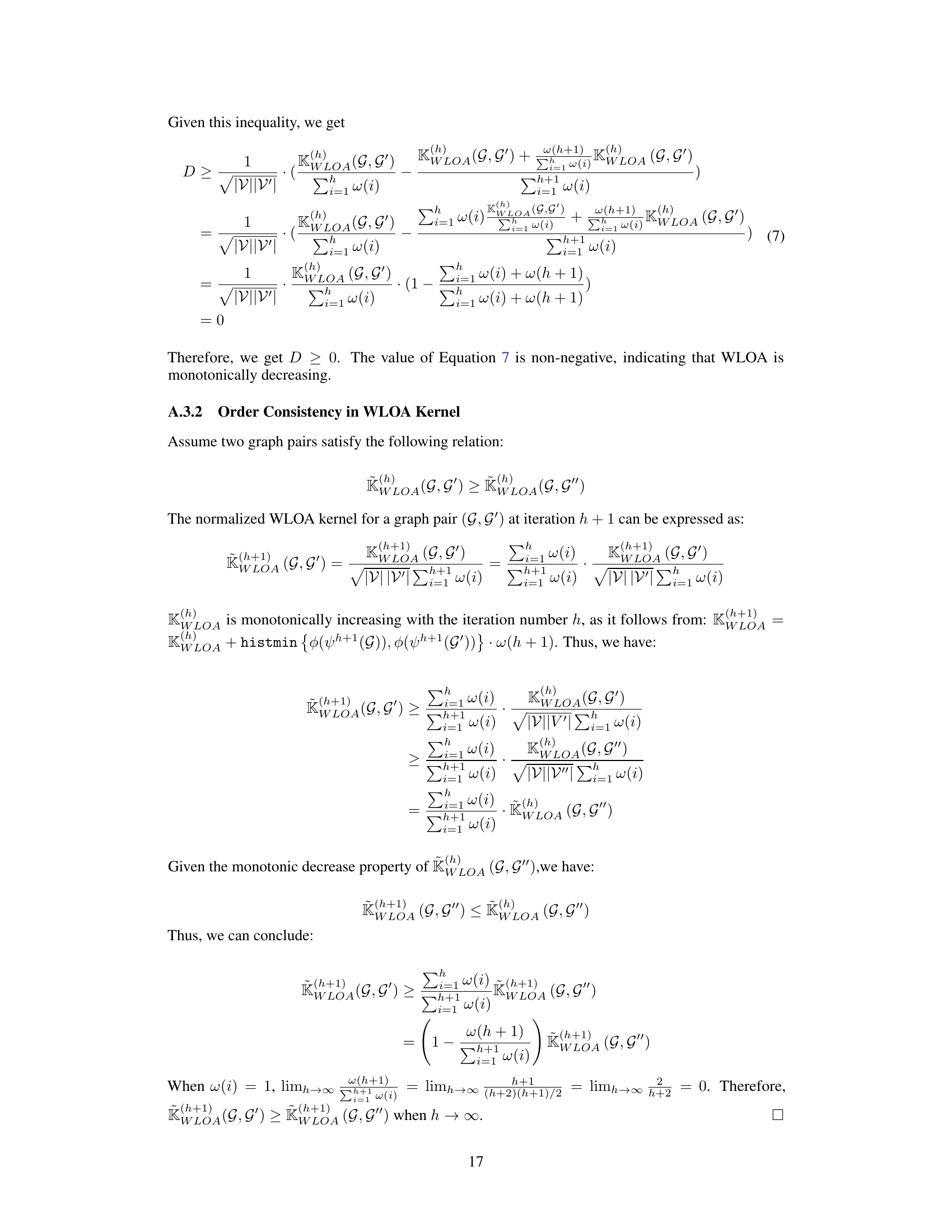
🔼 This table presents the statistics of the datasets used in the paper’s experiments. For each dataset, it shows the task it’s used for, the number of classes, the number of graphs, the average number of nodes and edges per graph, and whether node labels are available.
read the caption
Table 5: Dataset statistics.

🔼 This table presents the average training time per epoch for various Graph Neural Network (GNN) models, both with and without the proposed consistency loss, on the ogbg-molhiv dataset. The models are GCN, GIN, GraphSAGE, GTransformer, and GMT. The table showcases the computational overhead introduced by the consistency loss and allows for a comparison of training efficiency across different GNN architectures.
read the caption
Table 6: Average training time per epoch for different models on the ogbg-molhiv dataset, measured in seconds.

🔼 This table presents the peak memory usage (in MB) during training on the ogbg-molhiv dataset for various GNN models, both with and without the proposed consistency loss. It shows the memory consumption for each model and highlights the minimal increase in memory usage when the consistency loss is added, demonstrating the scalability of the method.
read the caption
Table 7: Peak memory usage for different models on the ogbg-molhiv dataset, measured in megabytes.

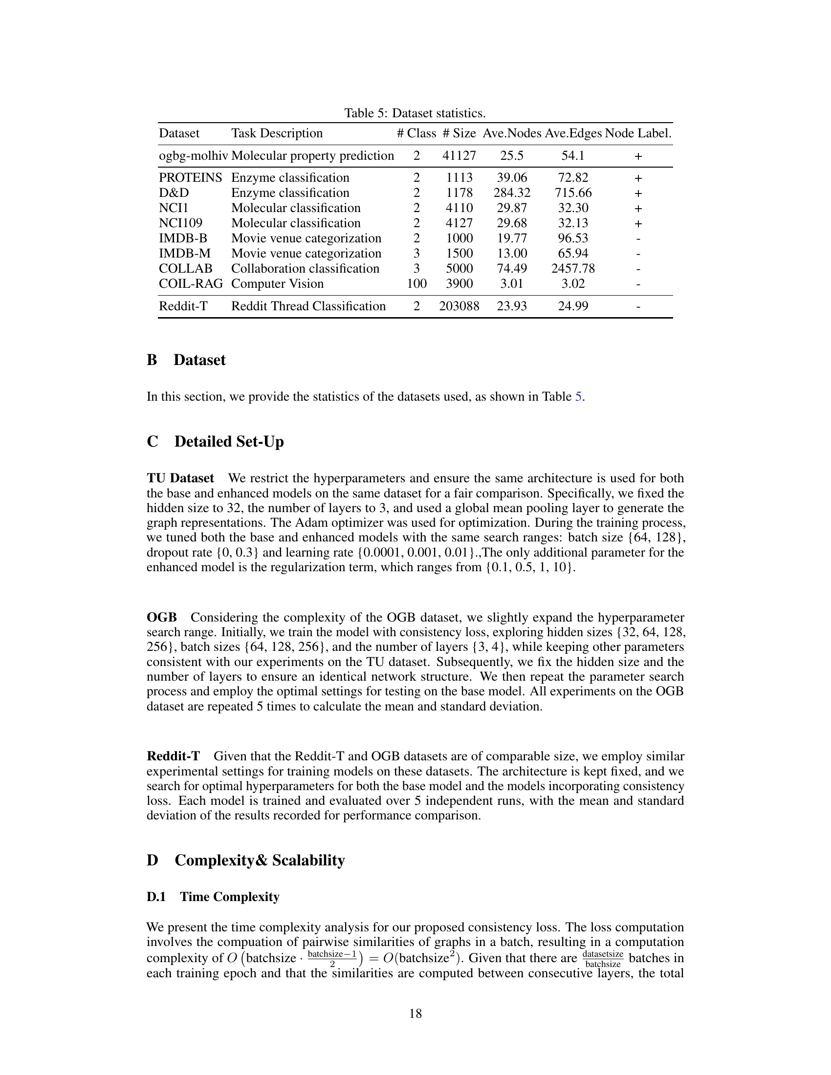
🔼 This table presents the average training time per epoch for different models on subsets of the REDDIT dataset with varying numbers of classes. The subsets consist of 2, 3, 4, and 5 classes, respectively. The table compares the training time of the baseline GCN model to the GCN model with the proposed consistency loss added. This allows the reader to assess the impact of increased task complexity and the consistency loss on training efficiency.
read the caption
Table 8: Average training time per epoch on REDDIT subsets with varying class complexity, measured in seconds

🔼 This table shows the average training time per epoch for three subsets of the IMDB-B dataset, each with a different level of structural complexity (small, medium, large). The training time is measured for both a standard GCN model and a GCN model enhanced with the proposed consistency loss. The table demonstrates that the added computational cost of the consistency loss remains minimal across datasets with varying structural complexity.
read the caption
Table 9: Average training time per epoch for subsets of varying structural complexity from IMDB-B, measured in seconds.

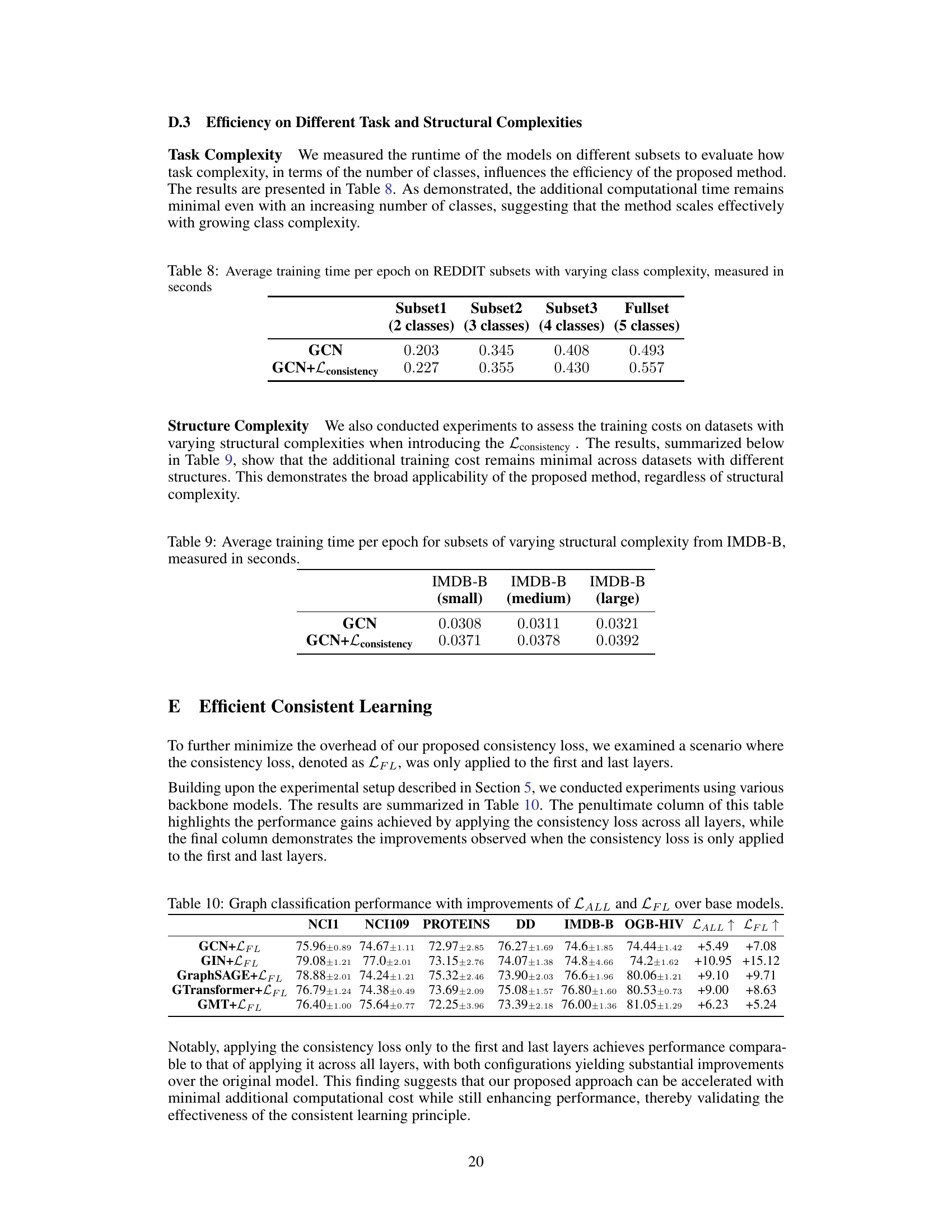
🔼 This table shows the performance improvements achieved by applying the consistency loss across all layers (LALL) and when applying it only to the first and last layers (LFL). It compares the performance gains on various datasets (NCI1, NCI109, PROTEINS, DD, IMDB-B, OGB-HIV) for different GNN models (GCN, GIN, GraphSAGE, GTransformer, GMT). The results demonstrate that applying the loss to only the first and last layers achieves comparable performance gains to applying it to all layers, indicating that the computational cost can be reduced while maintaining effectiveness.
read the caption
Table 10: Graph classification performance with improvements of LALL and LFL over base models.

🔼 This table presents the graph classification accuracy results achieved using a Graph Convolutional Network (GCN) model enhanced with contrastive learning (GCN+CL) and a GCN model enhanced with the proposed consistency loss (GCN+Lconsistency). The results are shown for several benchmark datasets, including NCI1, NCI109, PROTEINS, D&D, and IMDB-B. The table highlights the comparative performance of both methods across different datasets, illustrating the impact of the proposed consistency loss on classification accuracy.
read the caption
Table 11: Graph classification accuracy of GCN with contrastive learning applied across various datasets.

🔼 This table presents the Spearman rank correlation coefficients, measuring the consistency of graph similarity rankings across consecutive layers for different graph datasets (NCI1, NCI109, PROTEINS, D&D, IMDB-B). The results compare the consistency using Graph Contrastive Learning (GCN+CL) and the proposed consistency loss (GCN+Lconsistency). Higher correlation indicates greater consistency in similarity relationships across layers.
read the caption
Table 12: Spearman correlation for graph representations from consecutive layers.
Full paper#
