TL;DR#
Density-based spatial clustering of applications with noise (DBSCAN) is a powerful clustering algorithm but struggles with scalability in high-dimensional spaces due to its quadratic time complexity in identifying core points and neighborhoods. This limitation restricts its applicability to massive datasets frequently encountered in modern data analysis tasks. Existing approaches for scaling up DBSCAN either compromise accuracy or have limited theoretical guarantees.
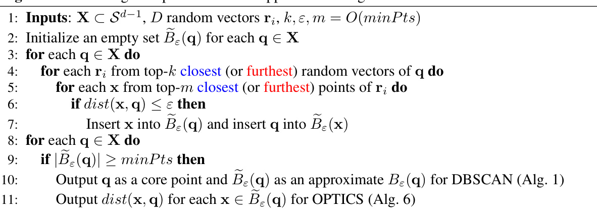
The researchers introduce sDBSCAN, which addresses these limitations by leveraging random projections to quickly identify core points and neighborhoods. This innovative method provably preserves the DBSCAN clustering structure under mild conditions, resulting in a significantly faster algorithm that achieves higher accuracy than existing alternatives. Moreover, the paper introduces sOPTICS, a scalable visual tool to guide parameter selection, making sDBSCAN more user-friendly and practically applicable to a wider range of problems. The empirical results on real-world datasets confirm the effectiveness of the proposed approach.
Key Takeaways#
Why does it matter?#
This paper is important because it presents sDBSCAN, a significantly faster and more accurate algorithm for density-based clustering, especially crucial for high-dimensional, large datasets. The method uses random projections to efficiently identify core points and their neighborhoods, overcoming the computational bottleneck of traditional DBSCAN. This work also introduces sOPTICS, a visual tool to guide parameter selection, further enhancing the usability and practical application of density-based clustering. These contributions are highly relevant to researchers working with big data and high-dimensional datasets across various domains, paving the way for more efficient and accurate cluster analysis.
Visual Insights#

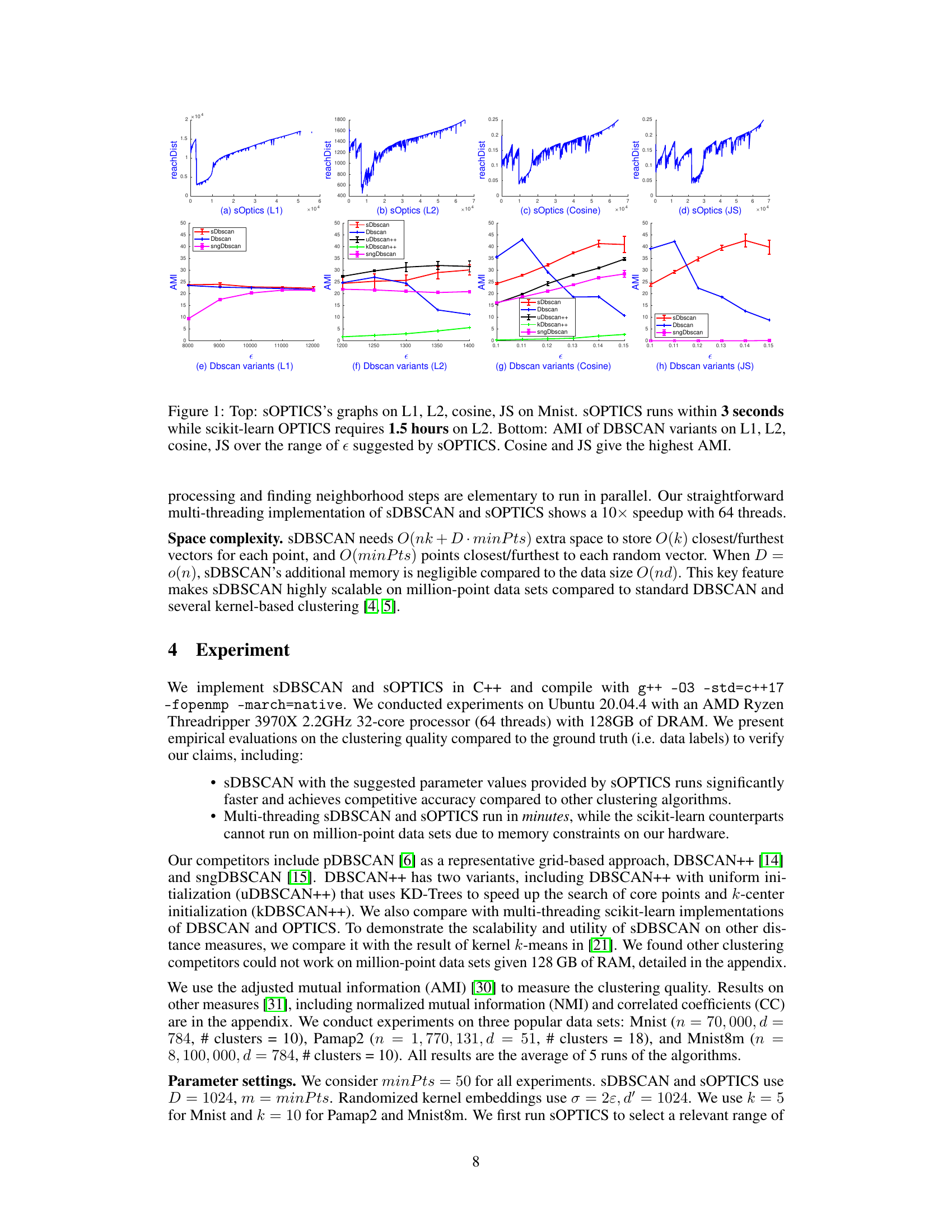
🔼 This figure shows the results of applying sOPTICS and several DBSCAN variants to the MNIST dataset. The top part displays the sOPTICS reachability plots for four different distance metrics: L1, L2, cosine, and Jensen-Shannon (JS). These plots visualize the density-based clustering structure and help guide the selection of the epsilon parameter for DBSCAN. The bottom part shows the Adjusted Mutual Information (AMI) scores for different DBSCAN variants across a range of epsilon values suggested by sOPTICS for each distance metric. The results show that sOPTICS is much faster than the scikit-learn OPTICS implementation and that the cosine and JS distance metrics generally provide the highest AMI scores.
read the caption
Figure 1: Top: sOPTICS's graphs on L1, L2, cosine, JS on Mnist. sOPTICS runs within 3 seconds while scikit-learn OPTICS requires 1.5 hours on L2. Bottom: AMI of DBSCAN variants on L1, L2, cosine, JS over the range of ɛ suggested by sOPTICS. Cosine and JS give the highest AMI.
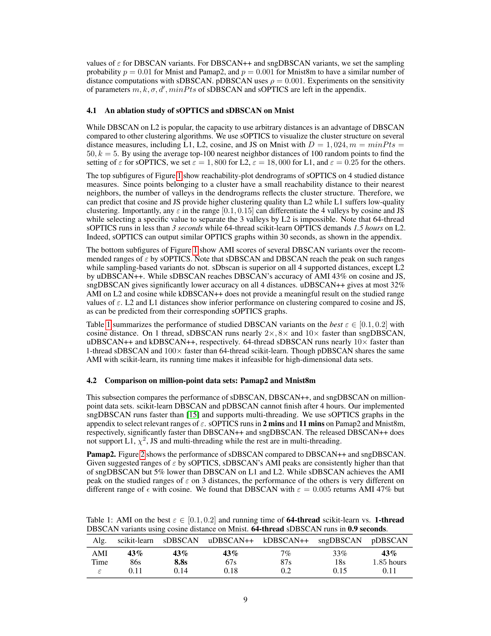
🔼 The table compares the Adjusted Mutual Information (AMI) scores and running times of different DBSCAN variants on the MNIST dataset using cosine distance. The best epsilon (ε) value within the range of 0.1 to 0.2 was used for each algorithm. The results highlight that sDBSCAN achieves comparable AMI to other methods but with significantly faster running times, especially when using multiple threads (64 threads for sDBSCAN vs. 1 thread for others).
read the caption
Table 1: AMI on the best ε ∈ [0.1, 0.2] and running time of 64-thread scikit-learn vs. 1-thread DBSCAN variants using cosine distance on Mnist. 64-thread sDBSCAN runs in 0.9 seconds.
In-depth insights#
sDBSCAN: Scalable DBSCAN#
The proposed sDBSCAN algorithm tackles the scalability challenges inherent in traditional DBSCAN, particularly in high-dimensional datasets. By cleverly leveraging random projections, sDBSCAN significantly accelerates the core point identification process, which is typically the computational bottleneck. This approach avoids the costly O(n²) complexity associated with traditional ε-neighborhood searches. Instead, sDBSCAN employs a lightweight indexing mechanism based on random projections, thereby significantly speeding up the clustering process. The algorithm’s efficiency is further enhanced by employing efficient data structures and parallelization techniques to process datasets containing millions of data points. The effectiveness of sDBSCAN is not only demonstrated through substantial speed improvements but also by maintaining high clustering accuracy compared to standard DBSCAN and its various optimized versions. The theoretical analysis provides confidence in sDBSCAN’s ability to preserve the essential clustering structure under mild conditions. The integration of a visual tool, sOPTICS, aids in parameter selection, thus addressing a common practical challenge with DBSCAN’s parameter sensitivity. In essence, sDBSCAN provides a compelling solution for large-scale density-based clustering, improving both efficiency and accuracy.
Random Projection Indexing#
Random projection indexing offers a scalable and efficient approach to approximate nearest neighbor search, crucial for speeding up high-dimensional clustering algorithms like DBSCAN. The core idea is to project high-dimensional data points onto a lower-dimensional space using randomly generated vectors. This significantly reduces computational costs associated with distance calculations. The effectiveness relies on the property that, with high probability, the relative distances between points are preserved in the lower-dimensional projection. However, this approximation introduces errors, potentially impacting the accuracy of the clustering. The choice of the number of random projection vectors is critical: too few may lead to significant distance distortion and clustering inaccuracies, while too many increase computational costs, negating the benefits of dimensionality reduction. Careful consideration of this trade-off is key to balancing computational efficiency and clustering accuracy. Furthermore, the theoretical guarantees of this method often depend on strong assumptions about the data distribution, which might not always hold in real-world datasets. Practical implementations often involve additional heuristics or optimizations to further improve efficiency or accuracy. Therefore, while promising for large datasets, random projection indexing requires careful parameter tuning and a keen understanding of its limitations to ensure reliable and accurate results.
sOPTICS: Visual Parameter Tuning#
The proposed ‘sOPTICS: Visual Parameter Tuning’ method is a crucial contribution, addressing the challenge of parameter selection in DBSCAN-family algorithms. Traditional DBSCAN relies heavily on the often-arbitrary selection of epsilon (ε) and minimum points (minPts), significantly impacting results. sOPTICS offers a scalable and visual solution, generating a reachability-distance plot that effectively guides parameter choice. This interactive visualization allows users to identify optimal ε values by visually inspecting density-based cluster structures. By analyzing the valleys in the reachability plot, users can confidently determine suitable parameter settings, avoiding tedious trial-and-error processes and improving the overall efficiency and accuracy of density-based clustering. The scalability of sOPTICS ensures its applicability to large datasets, where traditional methods often fail. Its integration with random projections further enhances performance, making it suitable for high-dimensional data. Overall, sOPTICS represents a significant advancement in density-based clustering, bridging the gap between theoretical understanding and practical usability.
Empirical Performance Evaluation#
An empirical performance evaluation section in a research paper should meticulously assess the practical effectiveness of a proposed method. It needs to go beyond simple comparisons, demonstrating a deep understanding of strengths and weaknesses. This would involve a selection of relevant and challenging datasets, carefully chosen to highlight the method’s capabilities and limitations in various contexts. Robust statistical measures must be employed to gauge performance, such as mean average precision or F1-score, ensuring the results are reliable and not merely artifacts of specific dataset characteristics. A key element is comparison against strong baselines, ideally including state-of-the-art methods and well-established alternatives. The results section needs to be presented clearly, using visualizations like charts and tables to illustrate performance across different metrics and datasets, and to highlight significant findings. In addition, the analysis must interpret the results with nuanced explanations. It should provide insights into the reasons behind the observed performance trends, such as computational costs, the effectiveness of certain algorithms in diverse situations, and limitations based on data distribution or other factors. Finally, the conclusion should summarize and interpret these findings, contextualizing them within the broader research landscape. A rigorous empirical analysis is crucial for establishing the real-world impact of a new method.
Theoretical Guarantees & Limitations#
The theoretical underpinnings of the proposed scalable DBSCAN algorithm (sDBSCAN) rest on the asymptotic properties of extreme order statistics, specifically leveraging random projections to efficiently approximate neighborhoods. A key guarantee is that, under mild conditions on the data distribution, sDBSCAN preserves the clustering structure of the original DBSCAN algorithm with high probability. This is a significant improvement over existing sampling-based approaches, which often rely on stronger assumptions. However, the theoretical guarantees are asymptotic, meaning they hold as the number of random projections tends to infinity. In practice, a finite number of projections is used, introducing a trade-off between computational efficiency and the strength of the theoretical guarantees. The choice of parameters, such as the number of random projections and the size of the approximate neighborhoods, also affects the performance and accuracy of sDBSCAN, and optimal settings depend on the data characteristics. Therefore, while sDBSCAN offers theoretical justification for its scalability, it’s crucial to acknowledge the limitations inherent in applying asymptotic results to finite datasets and to carefully consider parameter selection for optimal performance in practice.
More visual insights#
More on figures

🔼 This figure shows a comparison of sOPTICS and the scikit-learn version of OPTICS, highlighting the significant speed improvement achieved by sOPTICS (3 seconds vs. 1.5 hours for L2). The bottom part displays the Adjusted Mutual Information (AMI) scores for various DBSCAN algorithms across different distance metrics (L1, L2, cosine, JS) over a range of epsilon (ɛ) values determined by sOPTICS. The results indicate that the cosine and Jensen-Shannon (JS) distances yield the highest AMI scores.
read the caption
Figure 1: Top: sOPTICS's graphs on L1, L2, cosine, JS on Mnist. sOPTICS runs within 3 seconds while scikit-learn OPTICS requires 1.5 hours on L2. Bottom: AMI of DBSCAN variants on L1, L2, cosine, JS over the range of ɛ suggested by sOPTICS. Cosine and JS give the highest AMI.

🔼 The figure compares the performance of different DBSCAN variants and kernel k-means on the Mnist8m dataset. The Normalized Mutual Information (NMI) is plotted against the epsilon (ε) parameter, which is a key parameter in DBSCAN. sOPTICS was used to suggest a range of relevant epsilon values. The figure highlights that sDBSCAN and its 1-Nearest Neighbor (1NN) variant achieve comparable performance to kernel k-means, a significantly more resource-intensive method, while running significantly faster than other DBSCAN variants.
read the caption
Figure 3: NMI comparison of DBSCAN variants on L2, cosine, χ², and JS and kernel k-means on Mnist8m over a wide ranges of ɛ suggested by sOPTICS. sDBSCAN and sDBSCAN-1NN runs within 10 mins and 15 mins while sngDBSCAN demands nearly 1 hour. Kernel k-means (k = 10) [21] runs in 15 mins on a supercomputer of 32 nodes, each has 64 threads and 128 GB of DRAM.

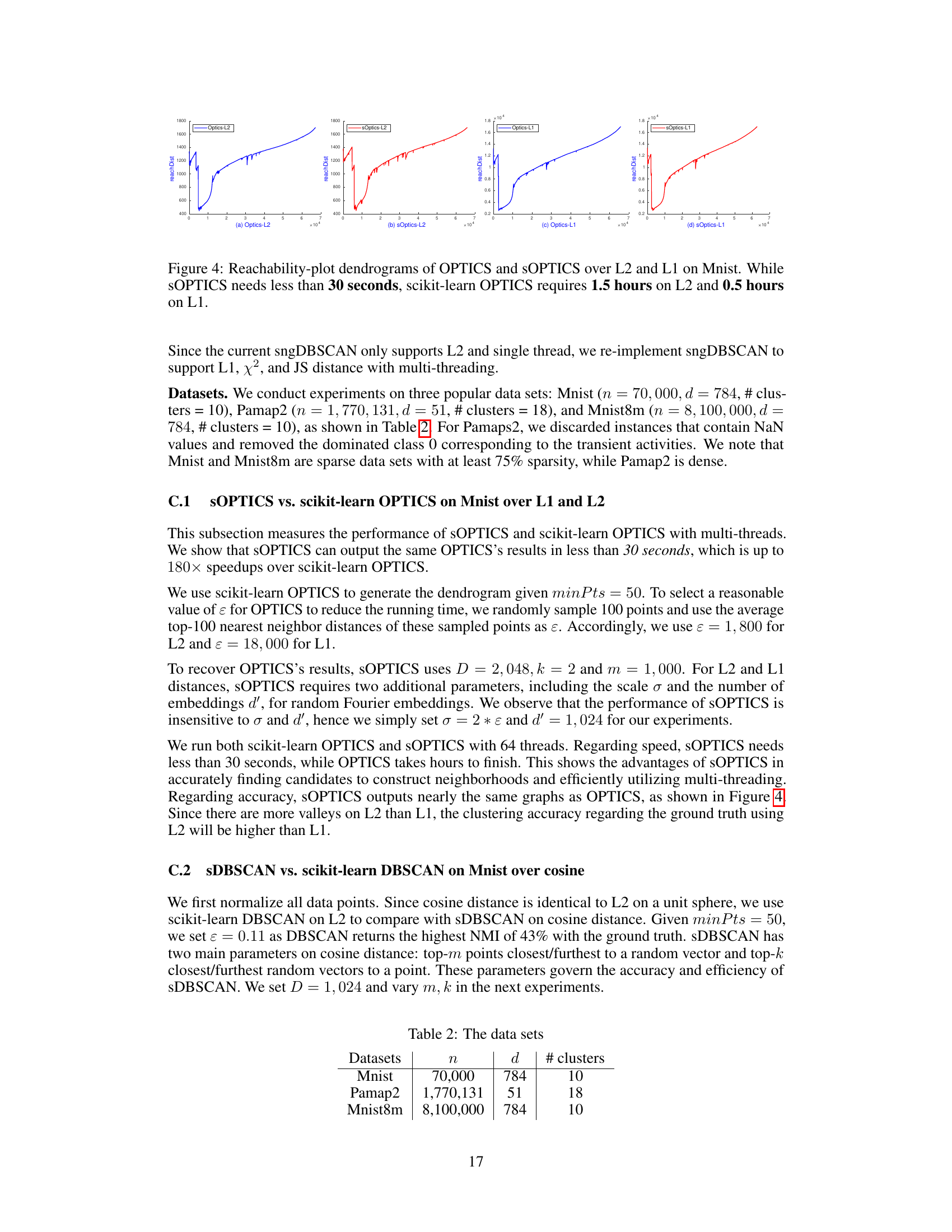
🔼 This figure compares the reachability plots generated by the OPTICS algorithm (from the scikit-learn library) and the proposed sOPTICS algorithm on the MNIST dataset. The plots visualize the density-based clustering structure for both L1 and L2 distance metrics. The key observation is the significant time difference: sOPTICS produces its results in under 30 seconds, while the standard OPTICS takes 1.5 hours for L2 and 0.5 hours for L1. The similarity in the shape of the curves indicates that sOPTICS effectively approximates the results of the original OPTICS algorithm.
read the caption
Figure 4: Reachability-plot dendrograms of OPTICS and sOPTICS over L2 and L1 on Mnist. While sOPTICS needs less than 30 seconds, scikit-learn OPTICS requires 1.5 hours on L2 and 0.5 hours on L1.

🔼 This figure compares the reachability plots generated by the standard OPTICS algorithm and the proposed sOPTICS algorithm for L1 and L2 distance metrics on the MNIST dataset. It highlights the significant speedup achieved by sOPTICS (less than 30 seconds) compared to the much longer runtime of the standard OPTICS algorithm (1.5 hours for L2 and 0.5 hours for L1). The reachability plots themselves visually represent the density-based clustering structure of the data, with valleys indicating cluster boundaries.
read the caption
Figure 4: Reachability-plot dendrograms of OPTICS and sOPTICS over L2 and L1 on Mnist. While sOPTICS needs less than 30 seconds, scikit-learn OPTICS requires 1.5 hours on L2 and 0.5 hours on L1.

🔼 The figure shows four reachability-plot dendrograms generated by OPTICS and sOPTICS algorithms on the MNIST dataset using L1 and L2 distances. The plots visualize the density-based clustering structure of the dataset. The key observation is that sOPTICS achieves comparable results to OPTICS significantly faster; sOPTICS takes less than 30 seconds, while the scikit-learn implementation of OPTICS takes 1.5 hours for L2 and 0.5 hours for L1.
read the caption
Figure 4: Reachability-plot dendrograms of OPTICS and sOPTICS over L2 and L1 on Mnist. While sOPTICS needs less than 30 seconds, scikit-learn OPTICS requires 1.5 hours on L2 and 0.5 hours on L1.

🔼 The figure shows the impact of the parameter σ (sigma) on the Normalized Mutual Information (NMI) scores achieved by the SDBSCAN algorithm. Two different distance metrics (L1 and L2) are used, and different values of σ are tested (50, 100, 200, 400). The x-axis represents the epsilon (ε) parameter, and the y-axis represents the NMI. Each data point in the graph represents a single run of SDBSCAN, which took less than 20 seconds to complete. The purpose is to show how sensitive the performance of SDBSCAN is to the parameter σ and to determine the optimal σ values for both L1 and L2 distances.
read the caption
Figure 7: SDBSCAN's NMI on L1 and L2 with various σ on Pamaps with k = 10, m = minPts = 50. Each runs in less than 20 seconds.

🔼 This figure shows the reachability plots generated by sOPTICS on the Pamap2 dataset using the L1 distance metric. Different plots represent different values of the parameter σ used in the random kernel feature mapping. The x-axis represents the point index in the linear ordering produced by sOPTICS, and the y-axis represents the reachability distance. The plots illustrate how the choice of σ affects the shape of the reachability plot and, consequently, the identification of clusters. The caption indicates that each plot was generated in under 2 minutes.
read the caption
Figure 8: SOPTICS's graphs on L1 with various σ on Pamaps with k = 10, m = minPts = 50. Each runs in less than 2 minutes.

🔼 The figure shows the reachability-plot dendrograms generated by OPTICS and sOPTICS algorithms for L2 and L1 distances on the MNIST dataset. It highlights the significant difference in computation time between the two methods; sOPTICS is substantially faster. The visual similarity of the dendrograms suggests that sOPTICS effectively approximates the results of OPTICS.
read the caption
Figure 4: Reachability-plot dendrograms of OPTICS and sOPTICS over L2 and L1 on Mnist. While sOPTICS needs less than 30 seconds, scikit-learn OPTICS requires 1.5 hours on L2 and 0.5 hours on L1.

🔼 This figure shows the Normalized Mutual Information (NMI) scores achieved by the sDBSCAN algorithm on the Pamap2 dataset using L1 and L2 distances. The experiment varies the parameter σ (sigma) in the random kernel mappings, while keeping k (number of closest/furthest random vectors) at 10 and m (number of closest/furthest points to each random vector) at 50 (equal to minPts). Each experimental run took less than 20 seconds to complete, demonstrating the efficiency of the sDBSCAN approach. The plots illustrate the sensitivity of the algorithm’s performance to the σ parameter and its optimal range for achieving high NMI scores on both L1 and L2 distance metrics.
read the caption
Figure 7: SDBSCAN's NMI on L1 and L2 with various σ on Pamaps with k = 10, m = minPts = 50. Each runs in less than 20 seconds.

🔼 This figure shows the reachability plots generated by sOPTICS for the chi-squared (x²) and Jensen-Shannon (JS) distance measures on the MNIST dataset. Two different values of d’ (the dimensionality of the random feature embedding) are compared: 3d and 5d, where d is the original dimensionality of the data. The plots visualize the reachability distance for each point, which helps to identify clusters and determine appropriate parameter settings for DBSCAN. The key observation is that sOPTICS with different values of d’ produce similar reachability plots, indicating the robustness of the method across varying embedding dimensionalities. Each plot was generated in under 3 seconds, showcasing the efficiency of the sOPTICS algorithm.
read the caption
Figure 11: sOPTICS's graphs on x² and JS with d' = {3d, 5d} on Mnist with k = 5, m = minPts = 50. Each runs in less than 3 seconds.

🔼 The figure shows the impact of parameters k and m on the Normalized Mutual Information (NMI) achieved by sDBSCAN on the Pamap2 dataset using the L1 distance. The parameter k represents the number of closest and furthest random vectors considered for each point, while m represents the number of closest and furthest points associated with each random vector. The figure presents two subplots: (a) k = 5 and (b) k = 10. Each subplot illustrates the NMI obtained by sDBSCAN with different values of m (50, 100, 200, 400) and varying epsilon (ε). The results demonstrate how choices for k and m affect the accuracy of sDBSCAN on this dataset. The x-axis represents the epsilon values, and the y-axis shows the NMI scores.
read the caption
Figure 12: sDBSCAN's NMI on L1 with various k, m on Pamaps with minPts = 50.

🔼 The figure shows the reachability plots generated by OPTICS and sOPTICS algorithms on the MNIST dataset using L1 and L2 distances. The plots visualize the density-based clustering structure. The key observation is the significant speedup achieved by sOPTICS (less than 30 seconds) compared to the scikit-learn implementation of OPTICS (1.5 hours for L2 and 0.5 hours for L1). The plots illustrate the differences in the reachability distances for different algorithms and distances, highlighting the efficiency of sOPTICS.
read the caption
Figure 4: Reachability-plot dendrograms of OPTICS and sOPTICS over L2 and L1 on Mnist. While sOPTICS needs less than 30 seconds, scikit-learn OPTICS requires 1.5 hours on L2 and 0.5 hours on L1.

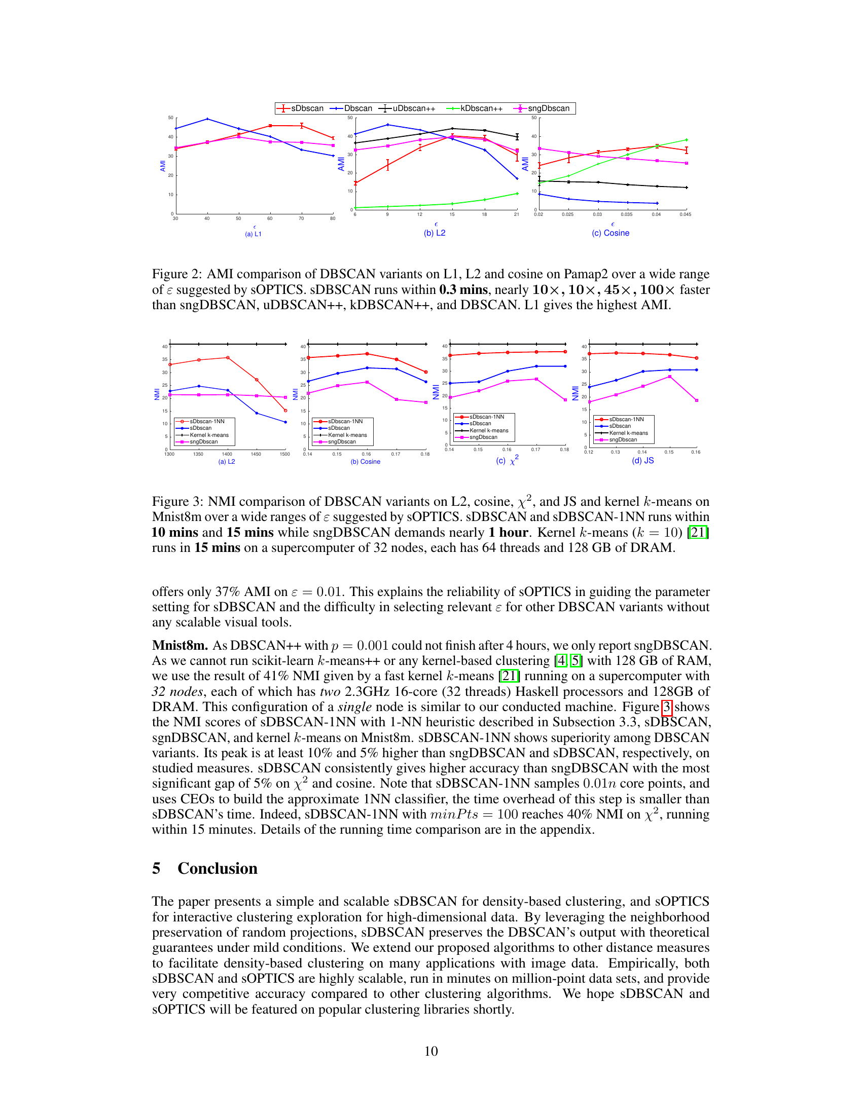
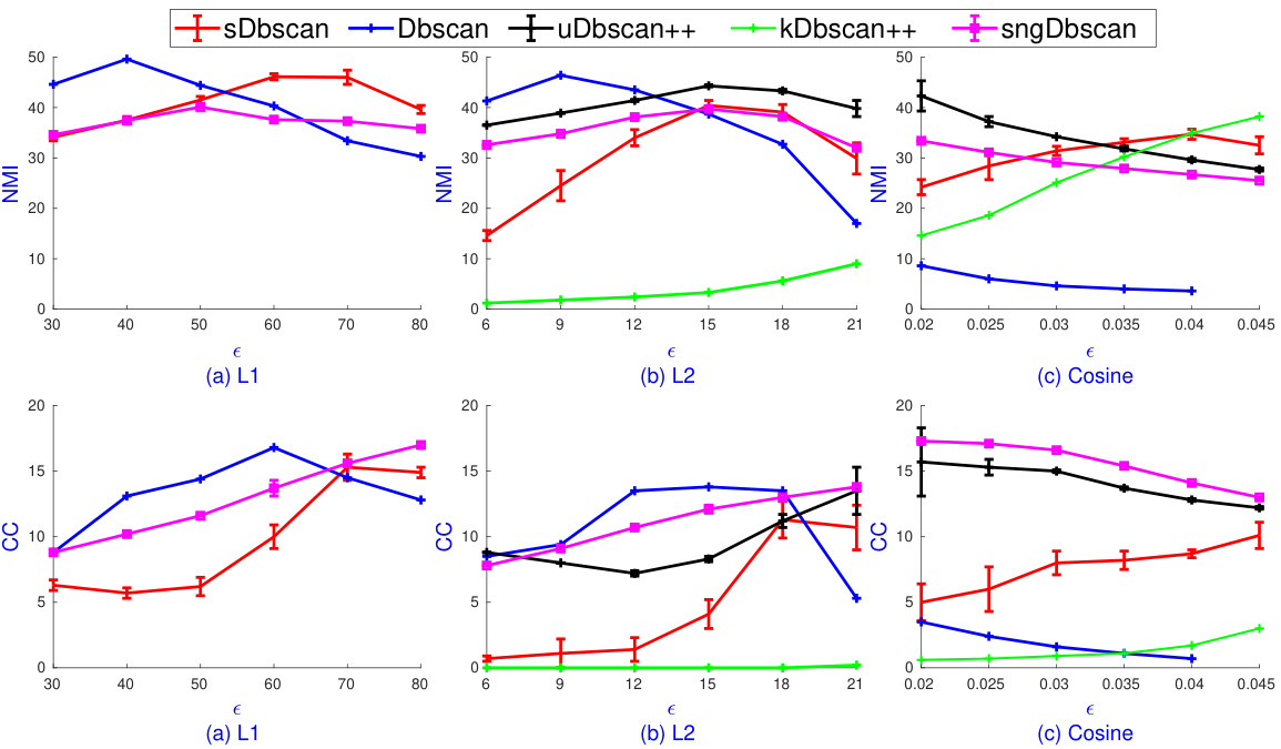
🔼 The figure compares the Adjusted Mutual Information (AMI) scores of different DBSCAN variants (sDBSCAN, DBSCAN, uDBSCAN++, kDBSCAN++, sngDBSCAN) on the Pamap2 dataset for L1, L2, and cosine distances across a range of epsilon (ε) values suggested by sOPTICS. The results show that sDBSCAN consistently achieves higher AMI scores than other algorithms, with L1 distance showing the highest AMI. Significantly, sDBSCAN demonstrates a significant speed improvement over the other variants, achieving a 10-100x speedup.
read the caption
Figure 2: AMI comparison of DBSCAN variants on L1, L2 and cosine on Pamap2 over a wide range of ε suggested by sOPTICS. sDBSCAN runs within 0.3 mins, nearly 10×,10×,45×,100× faster than sngDBSCAN, uDBSCAN++, kDBSCAN++, and DBSCAN. L1 gives the highest AMI.

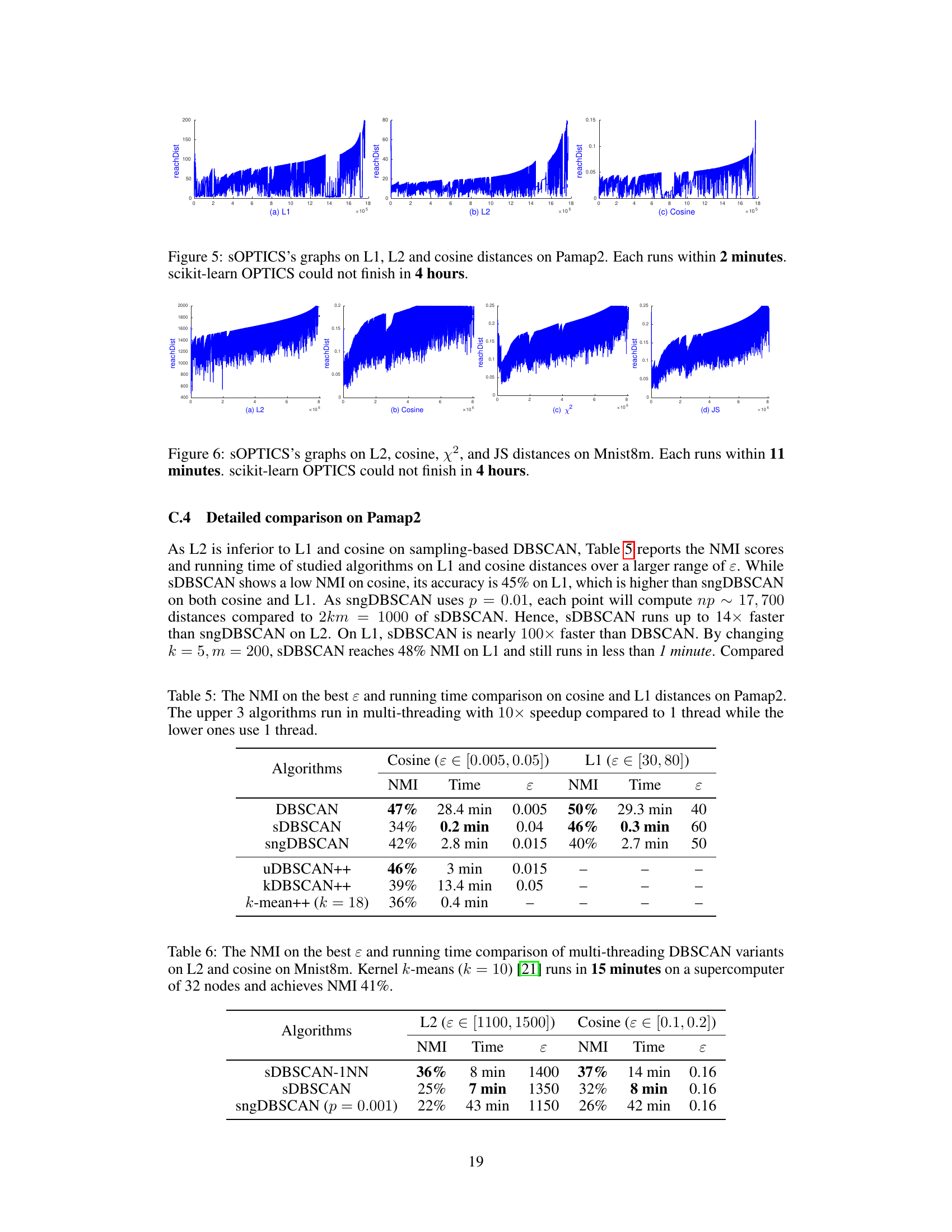
🔼 This figure shows the results of running sOPTICS on the Pamap2 dataset using L1, L2, and cosine distances. The key takeaway is that sOPTICS is significantly faster than the scikit-learn implementation of OPTICS, completing its analysis in just 2 minutes, while scikit-learn OPTICS failed to finish within 4 hours. This highlights the scalability of sOPTICS for large datasets.
read the caption
Figure 5: sOPTICS's graphs on L1, L2 and cosine distances on Pamap2. Each runs within 2 minutes. scikit-learn OPTICS could not finish in 4 hours.

🔼 This figure compares the normalized mutual information (NMI) scores achieved by four different algorithms (sDBSCAN-1NN, sDBSCAN, Kernel k-means, and sngDBSCAN) on the MNIST8m dataset using four different distance measures (L2, cosine, chi-squared, and Jensen-Shannon). The x-axis represents the epsilon (ε) parameter, and the y-axis represents the NMI score. The figure shows the performance of each algorithm across various values of ε for each distance measure. Each run took around 20 minutes.
read the caption
Figure 16: sDBSCAN's NMI on L2, cosine, x², and JS on Mnist8m with k = 10, m = minPts = 100. Each runs within 20 minutes.

🔼 The figure shows the results of applying sOPTICS and DBSCAN variants to the MNIST dataset using four different distance metrics (L1, L2, cosine, and Jensen-Shannon). The top part displays the reachability plots generated by sOPTICS, highlighting the efficiency of sOPTICS compared to the scikit-learn OPTICS (which takes significantly longer to produce similar results). The bottom part compares the Adjusted Mutual Information (AMI) scores of various DBSCAN implementations across the different distance metrics, showing that cosine and Jensen-Shannon distances yield the highest AMI scores.
read the caption
Figure 1: Top: SOPTICS’s graphs on L1, L2, cosine, JS on Mnist. SOPTICS runs within 3 seconds while scikit-learn OPTICS requires 1.5 hours on L2. Bottom: AMI of DBSCAN variants on L1, L2, cosine, JS over the range of ɛ suggested by sOPTICS. Cosine and JS give the highest AMI.
🔼 This figure shows the results of applying sOPTICS and comparing different DBSCAN variants. The top part displays reachability plots generated by sOPTICS for various distance measures (L1, L2, cosine, and Jensen-Shannon) on the MNIST dataset. It highlights the speed advantage of sOPTICS over scikit-learn OPTICS. The bottom part presents a comparison of the Adjusted Mutual Information (AMI) scores for several DBSCAN variants (sDBSCAN, DBSCAN, uDBSCAN++, kDBSCAN++, and sngDBSCAN) across the different distance measures. The epsilon (ε) values used were guided by the sOPTICS results. The results show that cosine and Jensen-Shannon distances yield the highest AMI scores.
read the caption
Figure 1: Top: SOPTICS's graphs on L1, L2, cosine, JS on Mnist. SOPTICS runs within 3 seconds while scikit-learn OPTICS requires 1.5 hours on L2. Bottom: AMI of DBSCAN variants on L1, L2, cosine, JS over the range of ε suggested by sOPTICS. Cosine and JS give the highest AMI.
More on tables

🔼 This table compares the Adjusted Mutual Information (AMI) scores and running times of different DBSCAN variants on the MNIST dataset using cosine distance. The best epsilon (ε) value within the range of [0.1, 0.2] was used for each algorithm. The table highlights that the proposed sDBSCAN algorithm achieves comparable accuracy to other methods while being significantly faster, especially when multi-threading is enabled.
read the caption
Table 1: AMI on the best ε ∈ [0.1, 0.2] and running time of 64-thread scikit-learn vs. 1-thread DBSCAN variants using cosine distance on Mnist. 64-thread sDBSCAN runs in 0.9 seconds.
🔼 This table compares the Adjusted Mutual Information (AMI) scores and running times of different DBSCAN variants on the MNIST dataset using cosine distance. The best epsilon (ε) value within the range of [0.1, 0.2] was used for each algorithm. The comparison includes the scikit-learn DBSCAN implementation (using 64 threads), and several scalable DBSCAN variants: sDBSCAN, uDBSCAN++, kDBSCAN++, and sngDBSCAN (all using 1 thread except sDBSCAN, which uses 64 threads). The results highlight sDBSCAN’s superior speed and competitive accuracy compared to other methods.
read the caption
Table 1: AMI on the best ε ∈ [0.1, 0.2] and running time of 64-thread scikit-learn vs. 1-thread DBSCAN variants using cosine distance on Mnist. 64-thread sDBSCAN runs in 0.9 seconds.

🔼 This table presents a comparison of the Adjusted Mutual Information (AMI) scores and running times for different DBSCAN variants on the MNIST dataset using cosine distance. The best epsilon (ɛ) value within the range of [0.1, 0.2] was selected for each algorithm. The results show that sDBSCAN achieves comparable AMI to other algorithms while being significantly faster, especially when using 64 threads. The scikit-learn DBSCAN implementation is shown for comparison but is significantly slower.
read the caption
Table 1: AMI on the best ɛ ∈ [0.1, 0.2] and running time of 64-thread scikit-learn vs. 1-thread DBSCAN variants using cosine distance on Mnist. 64-thread sDBSCAN runs in 0.9 seconds.

🔼 This table compares the Adjusted Mutual Information (AMI) score and running time of different DBSCAN algorithms on the MNIST dataset using cosine distance. The algorithms compared include the scikit-learn implementation, sDBSCAN, uDBSCAN++, kDBSCAN++, sngDBSCAN, and pDBSCAN. The best epsilon (ε) value for each algorithm within the range of [0.1, 0.2] is also reported. The results show that sDBSCAN achieves comparable AMI to the scikit-learn and pDBSCAN implementations while being significantly faster.
read the caption
Table 1: AMI on the best ε ∈ [0.1, 0.2] and running time of 64-thread scikit-learn vs. 1-thread DBSCAN variants using cosine distance on Mnist. 64-thread sDBSCAN runs in 0.9 seconds.

🔼 This table presents the characteristics of three datasets used in the experiments: Mnist, Pamap2, and Mnist8m. For each dataset, it lists the number of data points (n), the dimensionality (d), and the number of clusters.
read the caption
Table 2: The data sets

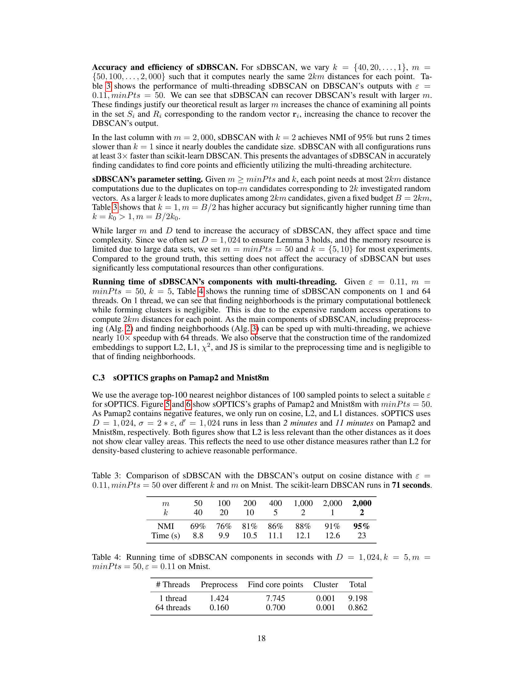
🔼 This table compares the accuracy (NMI) and efficiency (Time in seconds) of sDBSCAN with different combinations of parameters k and m against the original DBSCAN’s output (using cosine distance) on the MNIST dataset. It shows how increasing m (number of points considered) improves the NMI score, but also increases the runtime. The scikit-learn DBSCAN runtime of 71 seconds serves as a baseline for comparison.
read the caption
Table 3: Comparison of sDBSCAN with the DBSCAN's output on cosine distance with ε = 0.11, minPts = 50 over different k and m on Mnist. The scikit-learn DBSCAN runs in 71 seconds.

🔼 This table shows the running time of different components of the sDBSCAN algorithm on the Mnist dataset with specific parameter settings. The components include preprocessing, finding core points, and clustering. The table compares the running time for both 1 thread and 64 threads, highlighting the impact of multi-threading on the efficiency of the algorithm.
read the caption
Table 4: Running time of sDBSCAN components in seconds with D = 1,024, k = 5, m = minPts = 50, ε = 0.11 on Mnist.

🔼 This table compares the performance of various DBSCAN algorithms (DBSCAN, sDBSCAN, sngDBSCAN, uDBSCAN++, kDBSCAN++, and k-means++) on the Pamap2 dataset using cosine and L1 distances. The table shows the Normalized Mutual Information (NMI) score, which measures the accuracy of the clustering, and the running time for each algorithm. Note that the top three algorithms utilized multi-threading, resulting in significantly faster execution times compared to the single-threaded algorithms shown below.
read the caption
Table 5: The NMI on the best ε and running time comparison on cosine and L1 distances on Pamap2. The upper 3 algorithms run in multi-threading with 10x speedup compared to 1 thread while the lower ones use 1 thread.

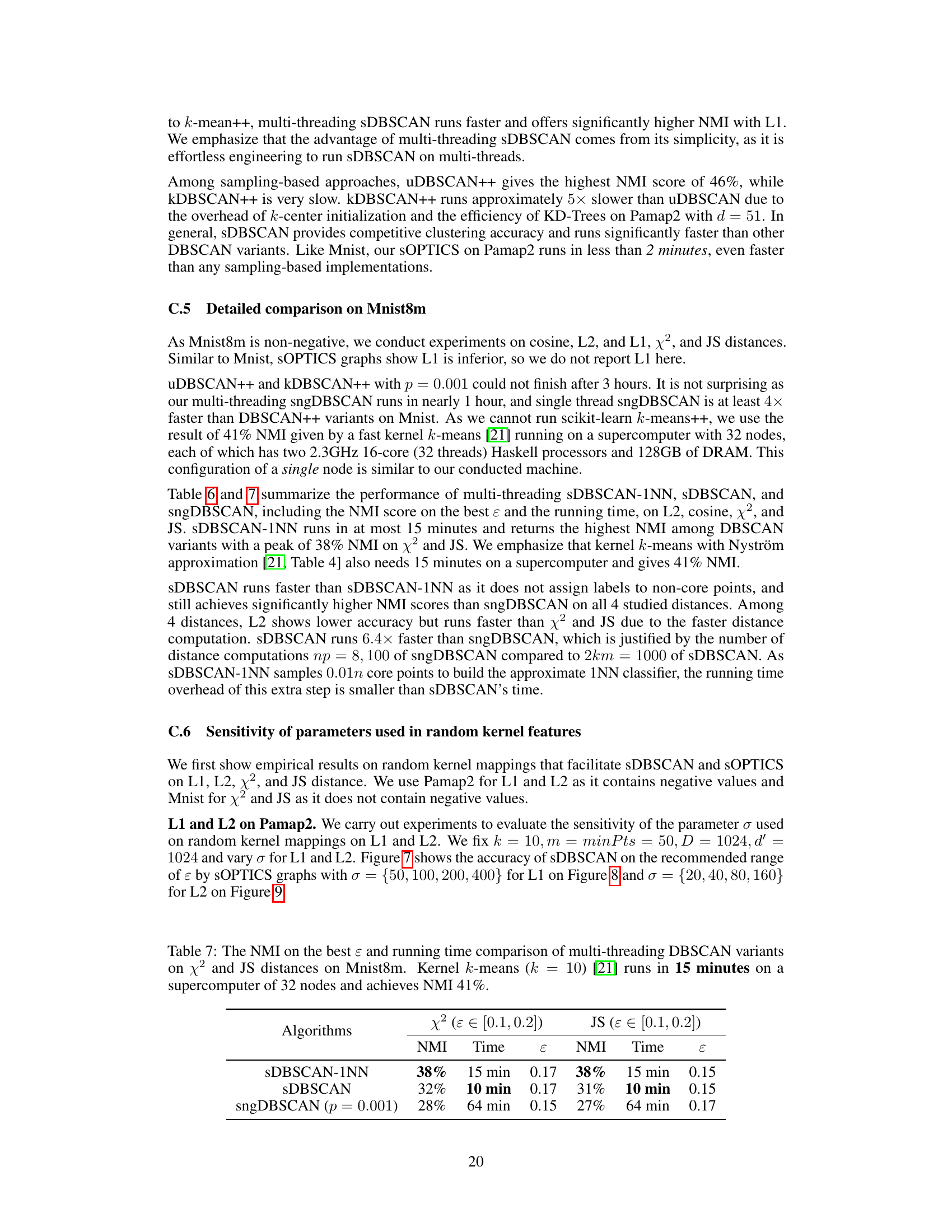
🔼 This table compares the performance of different DBSCAN variants (sDBSCAN-1NN, sDBSCAN, sngDBSCAN) and kernel k-means on the Mnist8m dataset using L2 and cosine distance. It shows the Normalized Mutual Information (NMI) achieved by each algorithm at their best epsilon (ε) value, along with their corresponding running times. The results highlight the superior speed of sDBSCAN and sDBSCAN-1NN compared to other methods, while demonstrating the competitiveness of sDBSCAN-1NN with the accuracy of the kernel k-means algorithm, which ran on a significantly more powerful supercomputer.
read the caption
Table 6: The NMI on the best ε and running time comparison of multi-threading DBSCAN variants on L2 and cosine on Mnist8m. Kernel k-means (k = 10) [21] runs in 15 minutes on a supercomputer of 32 nodes and achieves NMI 41%.

🔼 This table compares the performance of different DBSCAN variants (sDBSCAN-1NN, sDBSCAN, sngDBSCAN) and kernel k-means on the Mnist8m dataset using L2 and cosine distance metrics. It shows the Normalized Mutual Information (NMI) achieved by each algorithm at their optimal epsilon (ε) value and the time taken for each run. The results highlight sDBSCAN-1NN’s superior performance in terms of accuracy, while sDBSCAN achieves competitive results with significantly faster computation times compared to sngDBSCAN and kernel k-means.
read the caption
Table 6: The NMI on the best ε and running time comparison of multi-threading DBSCAN variants on L2 and cosine on Mnist8m. Kernel k-means (k = 10) [21] runs in 15 minutes on a supercomputer of 32 nodes and achieves NMI 41%.
Full paper#

