↗ OpenReview ↗ NeurIPS Homepage ↗ Chat
TL;DR#
Time series forecasting (TSF) models often struggle with long-range dependencies due to fixed-size inputs and the disruption of temporal correlations during minibatch training. This limitation significantly impacts prediction accuracy, especially for sequences with long-term trends.
To overcome this, the paper introduces Spectral Attention, a novel mechanism that preserves temporal correlations and efficiently handles long-range information. This is achieved by using a low-pass filter and an attention mechanism to preserve long-period trends and facilitate gradient flow between samples. Experiments on 11 real-world datasets show that Spectral Attention consistently outperforms existing methods, establishing new state-of-the-art results.
Key Takeaways#
Why does it matter?#
This paper is crucial for researchers working on time series forecasting because it directly addresses the critical challenge of capturing long-range dependencies, a problem that significantly limits the accuracy and effectiveness of existing models. The proposed Spectral Attention mechanism offers a novel, efficient solution, improving the state-of-the-art results across diverse datasets and models. Its model-agnostic nature allows for seamless integration into various forecasting architectures, opening new avenues for future research in enhanced long-term dependency modeling. This work’s efficacy and efficiency contribute to the advancement of forecasting accuracy in many critical real-world applications.
Visual Insights#

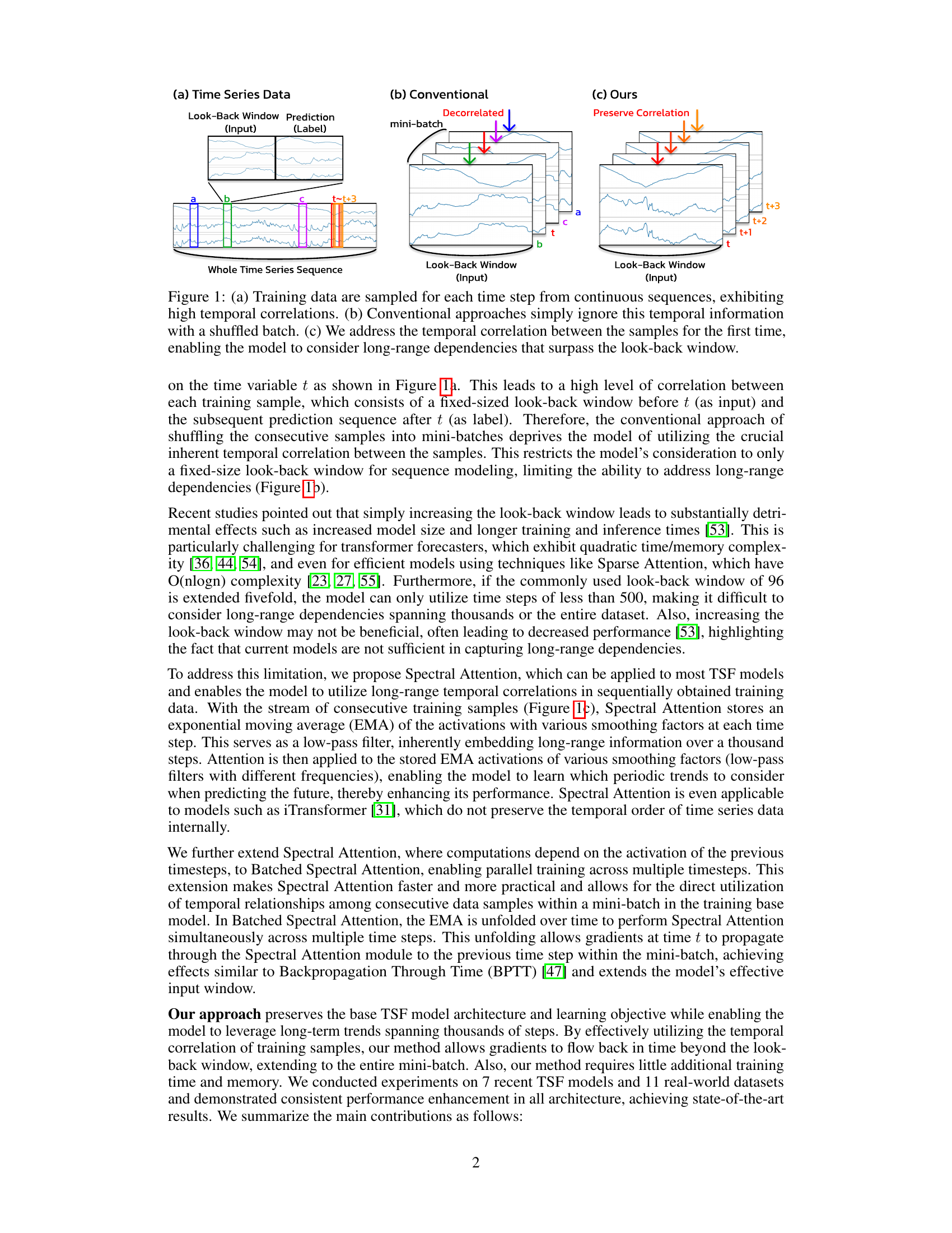
This figure illustrates the difference between conventional time series forecasting methods and the proposed approach. Panel (a) shows how time series data is naturally temporally correlated. Panel (b) shows how conventional methods shuffle the data, losing temporal correlations. Panel (c) shows the proposed method that preserves temporal correlation, enabling the capture of long-range dependencies.

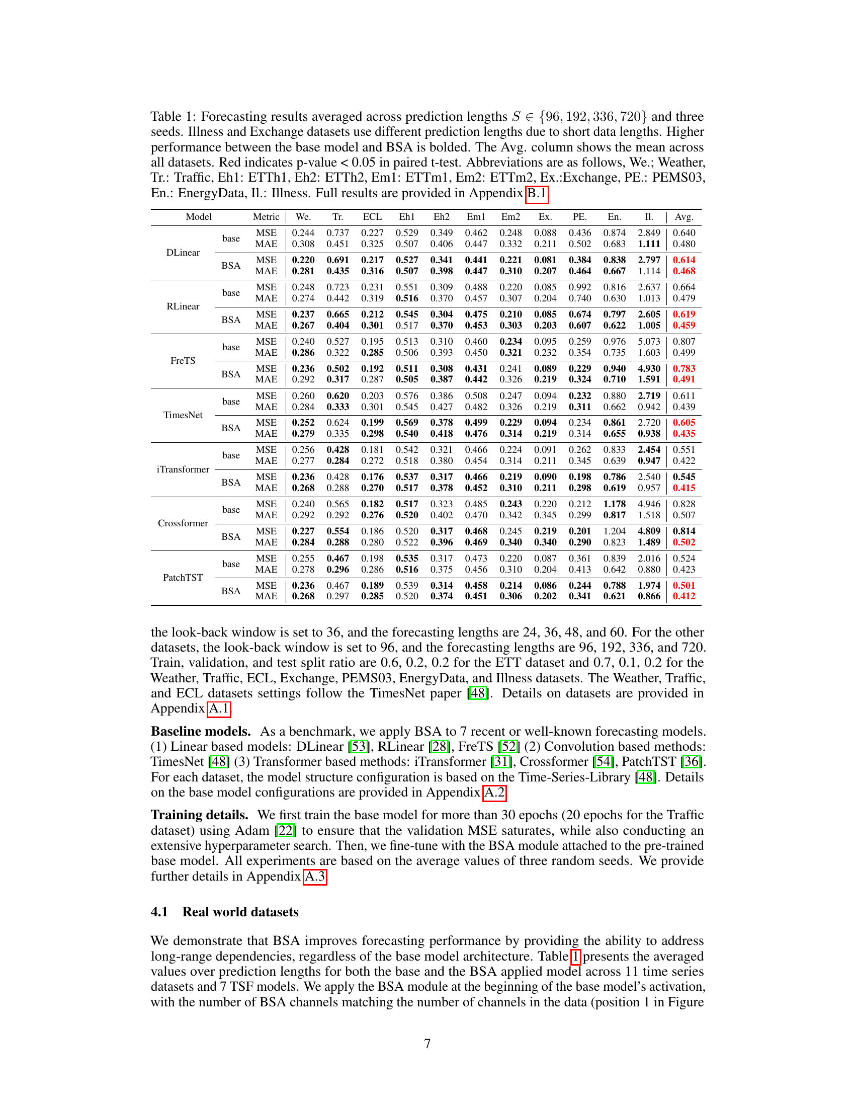
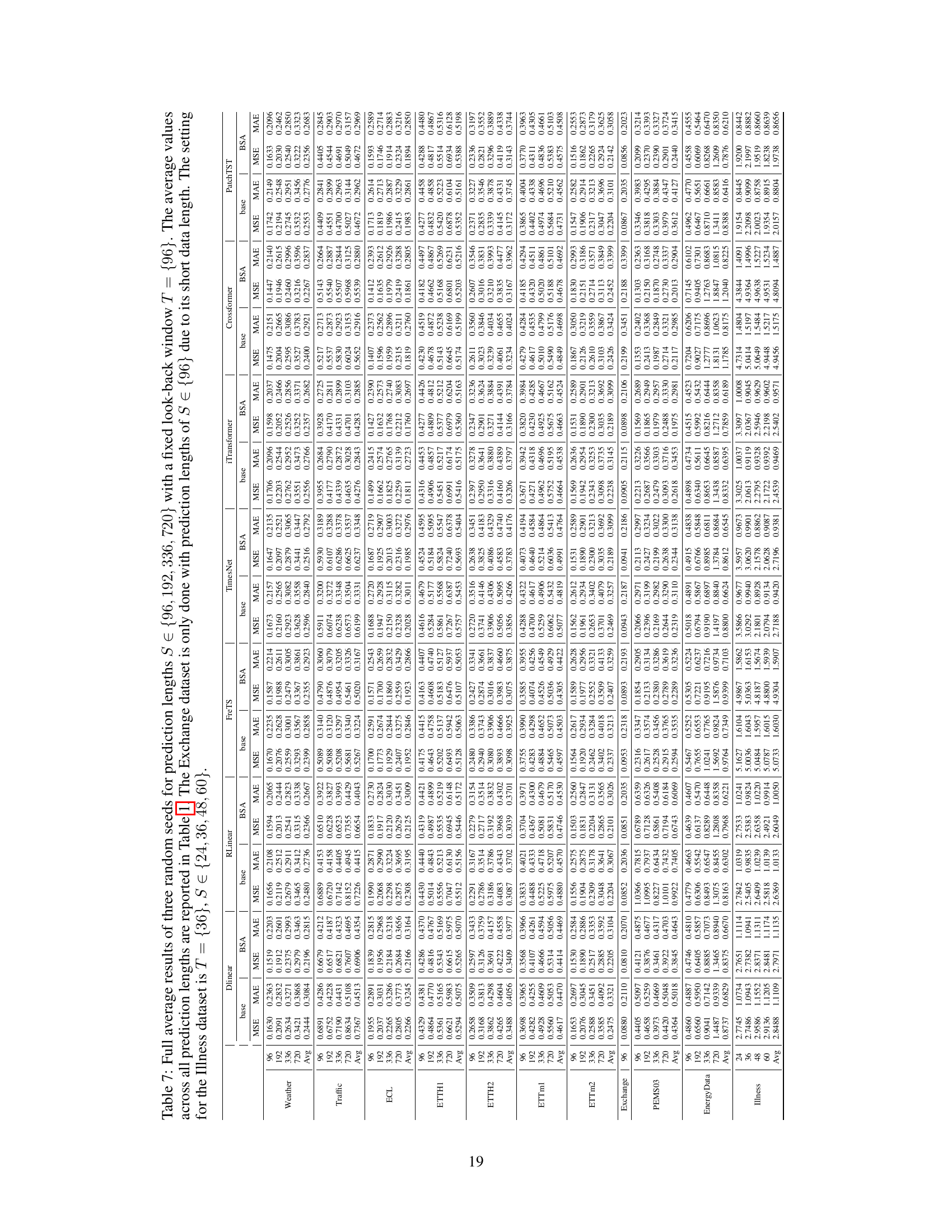
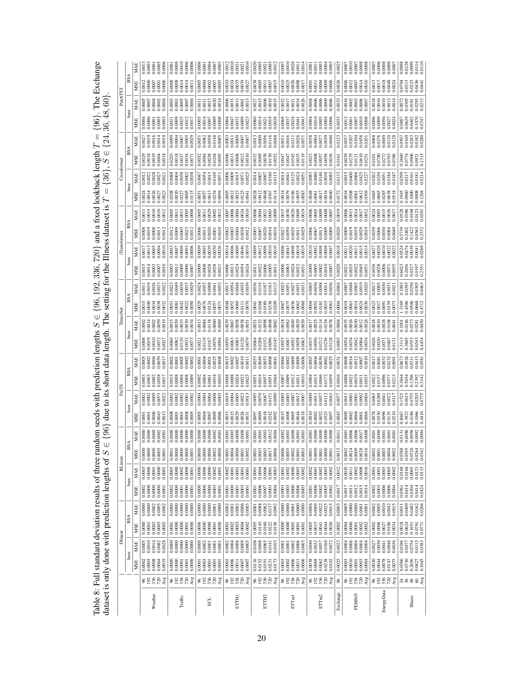
This table presents the average forecasting performance (MSE and MAE) of seven different time series forecasting models with and without the proposed BSA module across eleven real-world datasets. Different prediction lengths are used for some datasets due to their length. Statistical significance (p-value < 0.05) is indicated by red values, and bold values show where BSA improves upon baseline performance. The table averages results over three random seeds.
In-depth insights#
Spectral Attention#
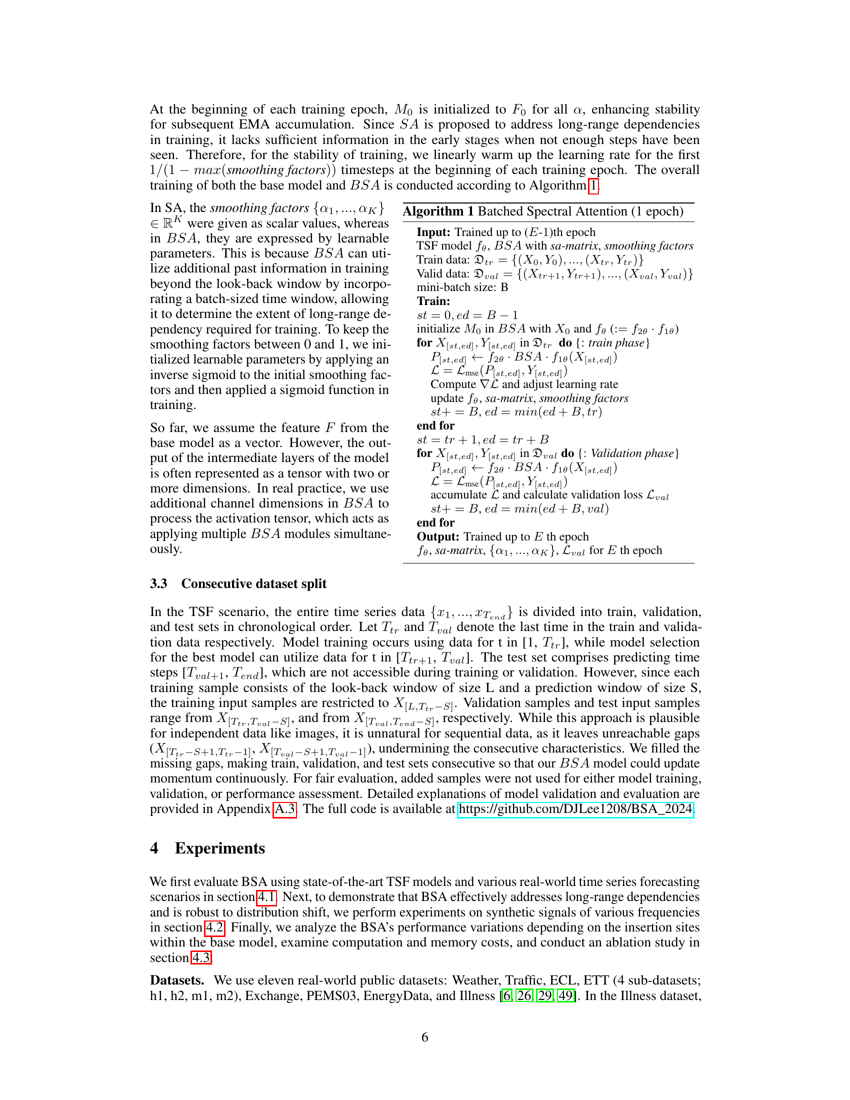
The proposed Spectral Attention mechanism is designed to enhance time series forecasting models by explicitly addressing long-range dependencies. It achieves this by preserving temporal correlations between training samples, unlike conventional methods that often shuffle data, losing valuable sequential information. The core idea involves employing a low-pass filter (exponential moving average) to capture long-term trends and high-frequency components, allowing the model to learn which periodic patterns to consider. This is integrated seamlessly into existing models, enhancing gradient flow across time and enabling the model to extend its effective input window beyond the fixed look-back limits. Batched Spectral Attention further improves efficiency by enabling parallel processing, further boosting the model’s ability to learn long-range temporal patterns. The authors demonstrate its efficacy across multiple models and datasets, consistently improving forecasting accuracy, particularly on datasets with substantial long-term trends. It’s key strength lies in its model-agnostic nature and minimal computational overhead.
Long-Range TSF#
Long-range time series forecasting (TSF) presents a significant challenge due to the inherent difficulty in capturing temporal dependencies that span extended periods. Traditional methods often struggle with this, leading to inaccurate predictions for longer time horizons. The core issue lies in the limitations of fixed-size input windows commonly used in models, preventing them from accessing and processing sufficiently distant past information to predict accurately far into the future. Advanced techniques, such as those based on transformers and spectral attention, are being explored to enhance long-range TSF performance. These aim to address the limitations of fixed-size windows and improve the modeling of long-term trends and seasonality, often by incorporating mechanisms to preserve and effectively utilize temporal correlations within the data. The effectiveness of these approaches relies on maintaining information flow between distant time steps, something that standard models frequently fail to achieve. Ultimately, the goal is to create models capable of producing accurate forecasts over vastly extended time horizons, which is crucial for many applications across various domains.
Model-Agnostic#
The term ‘Model-Agnostic’ in the context of a research paper typically signifies that the proposed method or technique is independent of the underlying model architecture. This implies broad applicability, as the approach can be integrated with various existing models without requiring significant modifications. A model-agnostic method’s effectiveness stems from its ability to enhance core functionalities, such as improving the handling of long-range dependencies or enhancing attention mechanisms, that are beneficial regardless of the base model’s specific design. This characteristic promotes wider adoption and facilitates straightforward integration into existing workflows, making it a more versatile and valuable contribution to the field. The absence of model-specific constraints often results in a greater impact, as the innovation can benefit a wider range of machine learning tasks and techniques. Generalizability and ease of implementation are key benefits of model-agnostic methods.
BSA Mechanism#
The Batched Spectral Attention (BSA) mechanism is a novel approach for enhancing time series forecasting models by explicitly addressing long-range dependencies. BSA cleverly integrates exponential moving averages (EMA) with various smoothing factors to maintain temporal correlations while simultaneously attending to multiple frequency components of the input data. This low-pass filtering effect, enabled by the EMA, preserves long-period trends. Crucially, the batched nature of BSA facilitates parallel training across multiple time steps, overcoming the computational limitations often encountered when increasing lookback windows. This enables gradient flow across mini-batches, mimicking the effectiveness of Backpropagation Through Time, thereby expanding the model’s effective temporal receptive field and enabling the capture of long-range dependencies. The seamless integration of BSA into most sequence models makes it a highly versatile and powerful tool for improving forecasting accuracy. Its efficacy is demonstrated through consistent improvements on diverse real-world datasets.
Future Works#
A future work section for this paper on Spectral Attention for long-range time series forecasting could explore several promising avenues. Extending Spectral Attention to other sequence model architectures beyond those tested would demonstrate its broader applicability and versatility. Investigating the impact of different smoothing factor selection strategies on model performance could reveal optimal parameterization techniques. Additionally, a comprehensive ablation study focusing on the interaction between Spectral Attention and other attention mechanisms within the model would yield valuable insights into their complementary roles and potential for synergistic improvement. Finally, applying the method to more diverse and challenging real-world datasets, especially those with irregular sampling or noisy data, would further validate its robustness and practical utility, while also uncovering potential limitations.
More visual insights#
More on figures
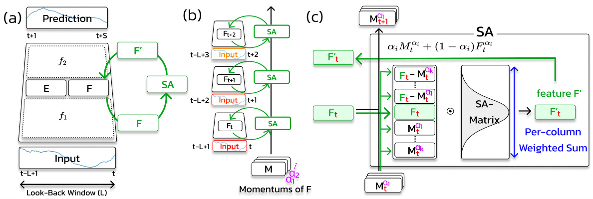
This figure illustrates the Spectral Attention (SA) module’s architecture and functionality. Panel (a) shows how the SA module is integrated into a time series forecasting model. Panel (b) shows the mechanism by which the SA module stores momentums of the feature vector to capture long-range dependencies, using multiple momentum parameters to capture dependencies across various ranges. Finally, panel (c) illustrates how the SA module computes the output vector F’ by attending to multiple low-frequency and high-frequency components of the feature vector F, using a learnable spectral attention matrix.

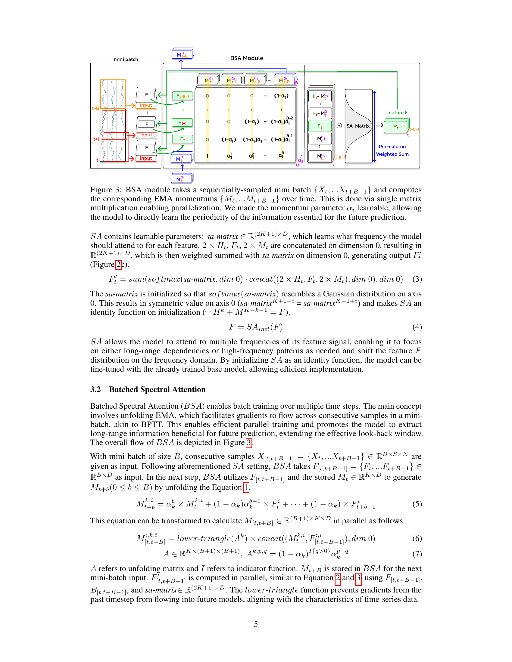
This figure illustrates the Batched Spectral Attention (BSA) module. The BSA module processes a mini-batch of sequentially sampled time series data, rather than shuffling the data as in conventional methods. It calculates exponential moving averages (EMA) of activations across multiple time steps within a mini-batch using a single matrix multiplication, enabling efficient parallelization. Notably, the momentum parameter (αi) is made learnable, allowing the model to dynamically adjust its sensitivity to different periodic patterns in the data for improved forecasting accuracy. This approach preserves temporal correlations and enables the model to capture long-range dependencies that surpass the look-back window.

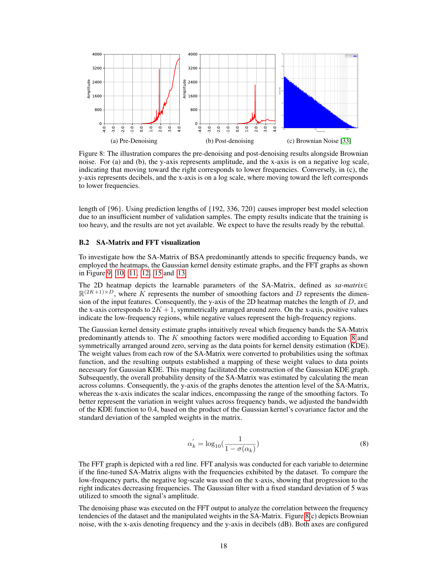
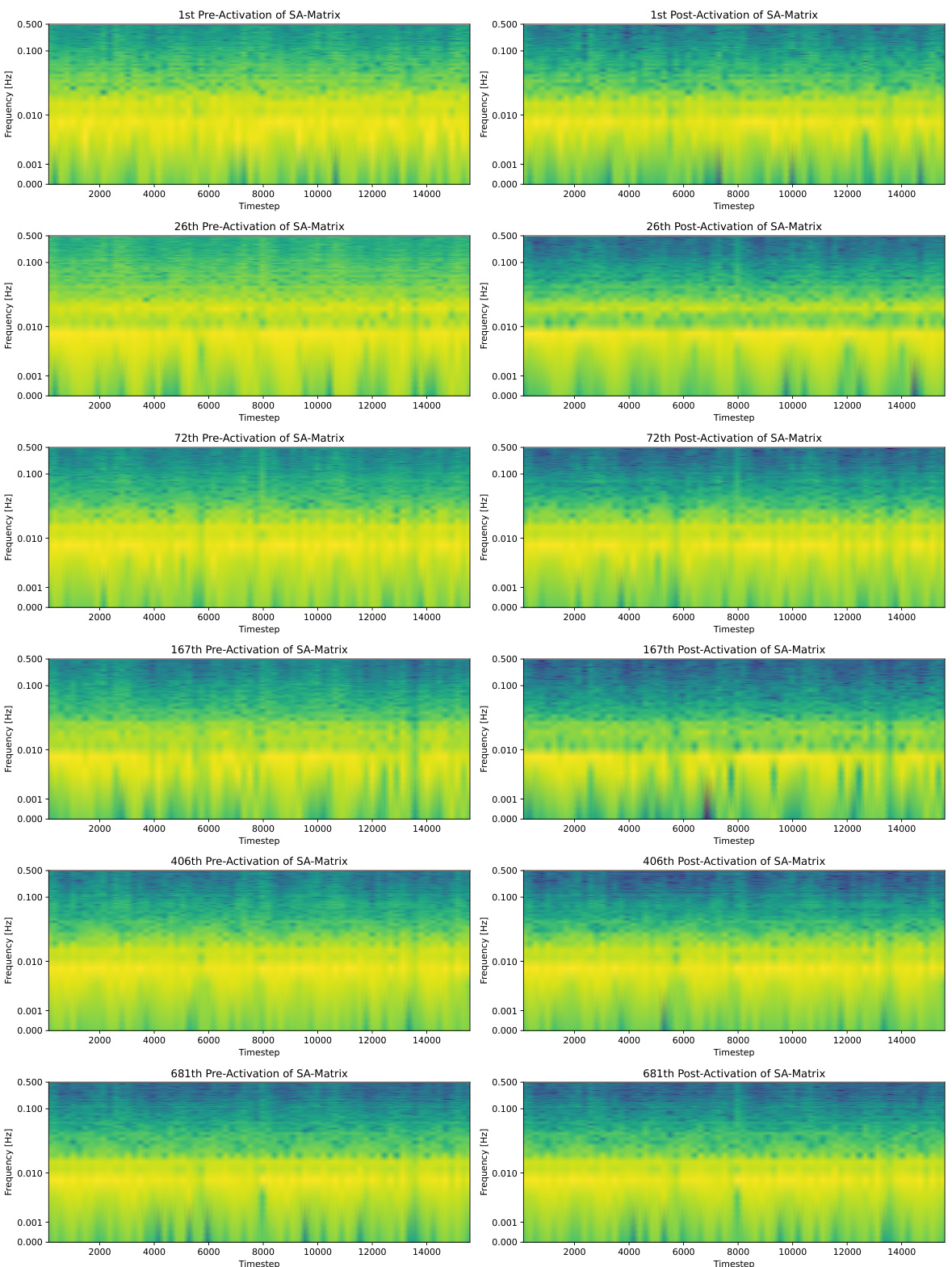
This figure visualizes the analysis of the spectral attention (SA) matrix from a DLinear model trained for a 720-step prediction task on Weather and ETTh1 datasets. Panel (a) presents a heatmap of the SA matrix, while panels (b), (c), and (d) display the attention and Fast Fourier Transform (FFT) graphs for specific channels within each dataset. These graphs help to illustrate how the SA module focuses on different frequency components for prediction and highlights the model’s ability to capture long-range dependencies.
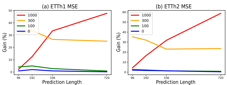
This figure shows the performance improvement of the iTransformer model with BSA on synthetic datasets created by adding sine waves with different periods (100, 300, 1000) to the original ETTh1 and ETTh2 datasets. The x-axis represents the prediction length, and the y-axis shows the percentage improvement in MSE compared to the base model (no BSA). Each line represents a different sine wave period, with ‘0’ representing the original dataset without added sine waves.

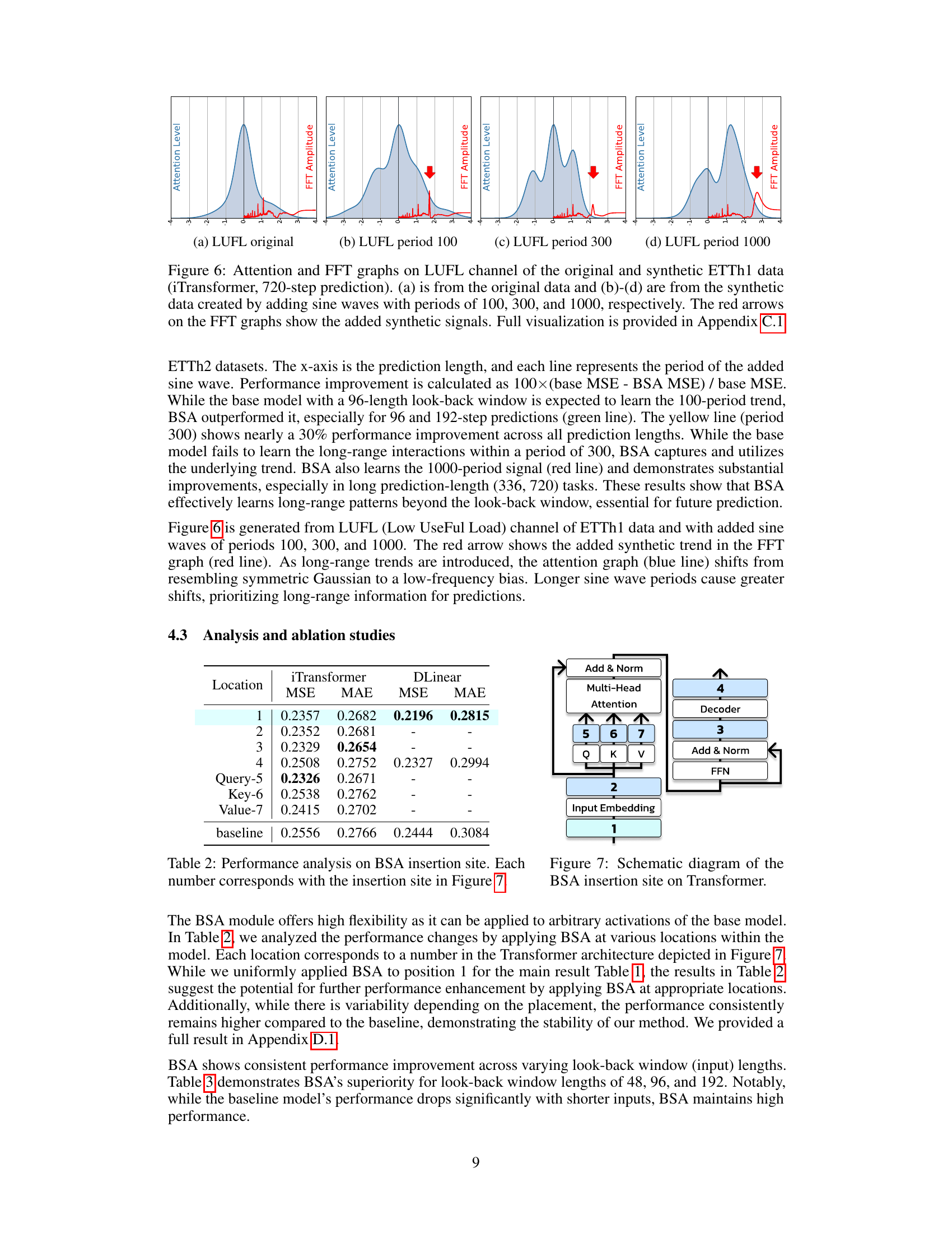
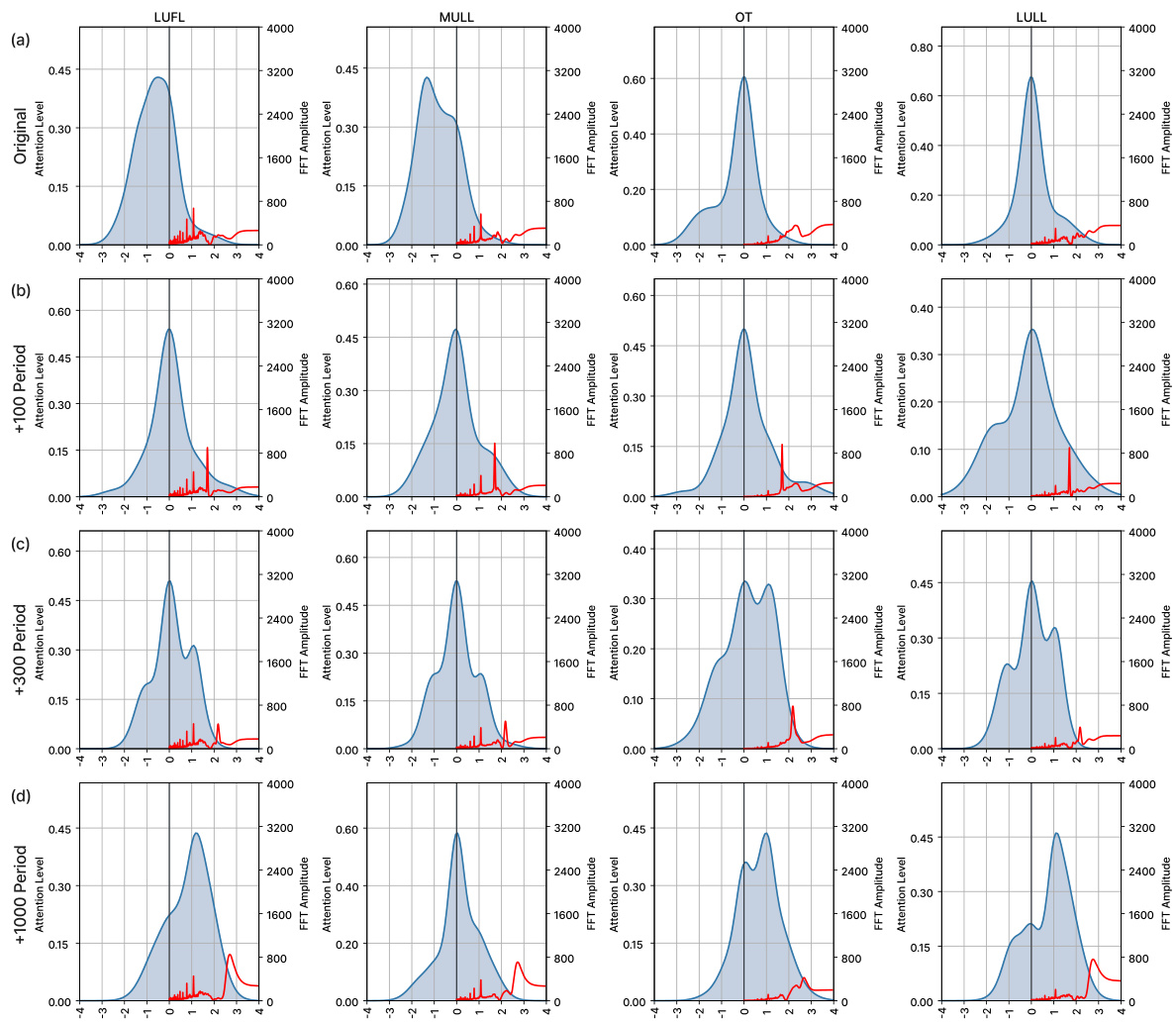
This figure presents a comparative analysis of the attention and FFT graphs for the LUFL channel of the ETTh1 dataset, both in its original form and with added sine waves of varying periods (100, 300, and 1000). The analysis uses the iTransformer model with a 720-step prediction. The red arrows in the FFT graphs highlight the added sine wave frequencies. The purpose is to show how the proposed BSA method effectively captures and utilizes long-range patterns, even those beyond the look-back window. This is evident in the changes in both the attention and FFT graphs as longer sine wave periods are included.
This figure shows the architecture of the Spectral Attention (SA) module. The SA module takes as input a subset of intermediate features from the base model and outputs features F’ which contains long-range information beyond the look-back window. The figure illustrates the mechanism through which the SA module achieves this: (a) The SA module is a plug-in module, meaning it can be inserted into the model without modifying the base architecture. Gradients flow through the SA module during training. (b) To capture long-range dependencies, the SA module stores the momentum of the feature vector F from sequential inputs. Multiple momentum parameters with different smoothing factors capture dependencies across various ranges. (c) The SA module calculates F’ by attending to multiple low-frequency and high-frequency components of F, using a learnable Spectral Attention Matrix.

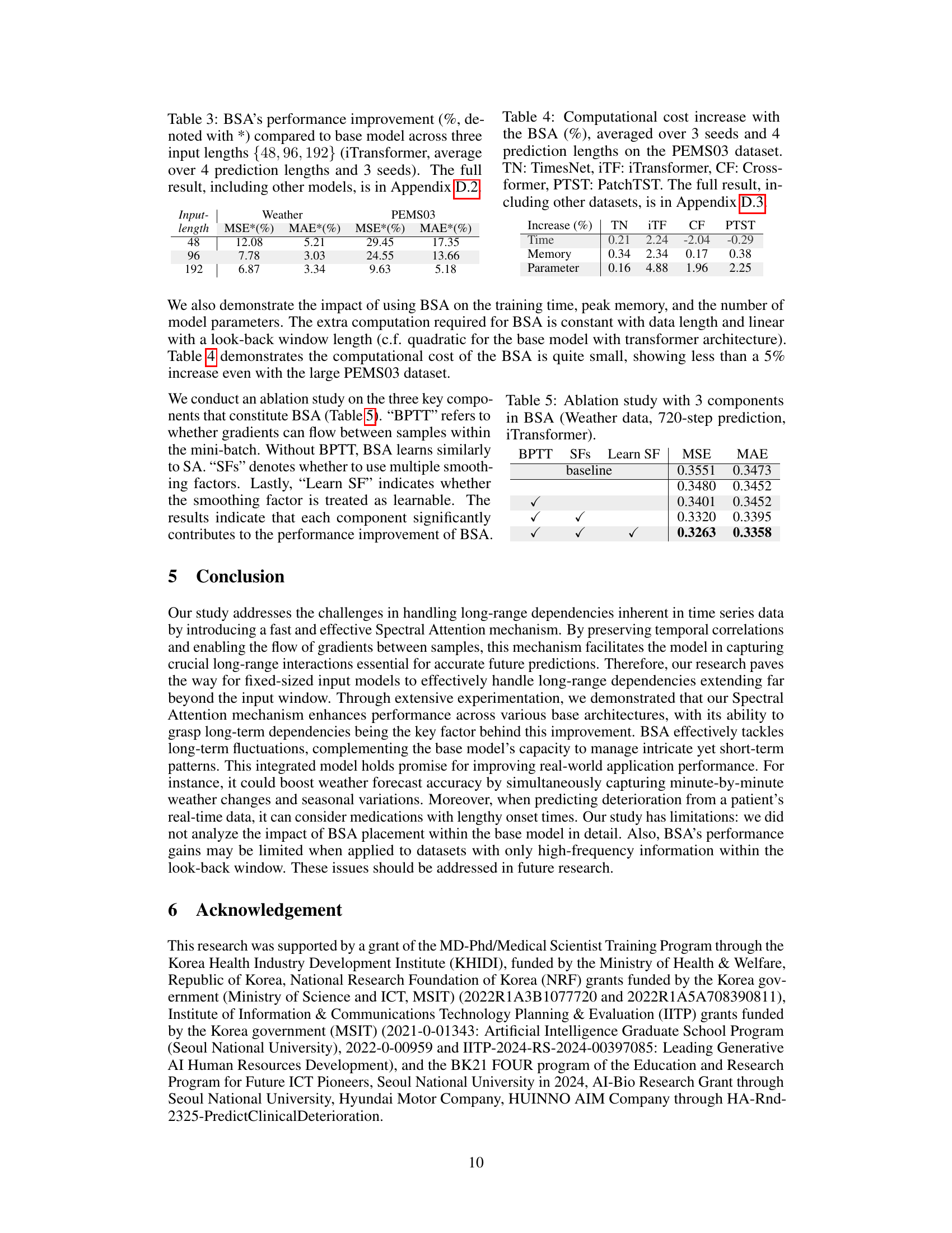
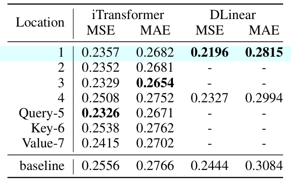
This figure shows the various locations within the Transformer model architecture where the Batched Spectral Attention (BSA) module can be inserted. The numbers 1 through 7 indicate specific layers or blocks within the transformer, such as Input Embedding, Multi-Head Attention, and Feed Forward Network (FFN) layers. The BSA module’s flexibility allows it to be integrated at different points within the model’s architecture, impacting its ability to influence the flow of information and gradient information within the network.

This figure shows the analysis of the SA-matrix of the DLinear model for long-range dependency prediction. Panel (a) visualizes the SA-matrix as a heatmap. Panels (b), (c), and (d) present the attention and FFT graphs for Weather Temperature, Weather Solar radiation, and ETTh1 Hull, respectively. The graphs illustrate how Spectral Attention focuses on low-frequency components, effectively capturing long-range dependencies.
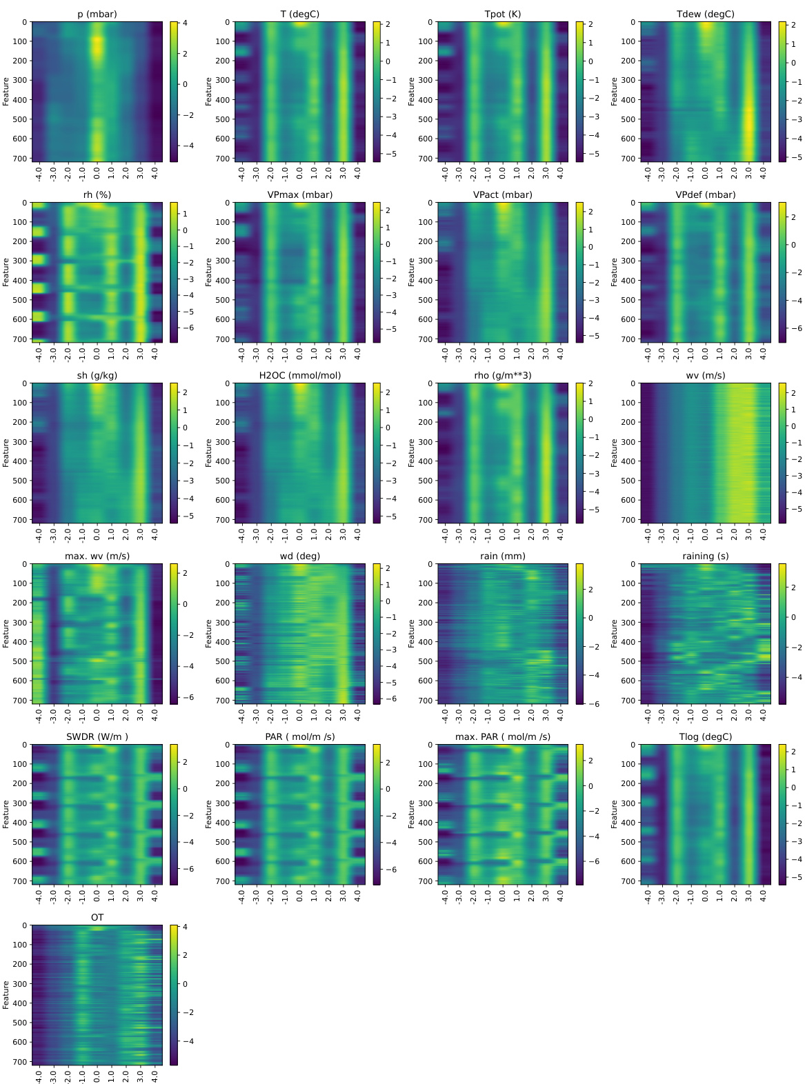
This figure provides a detailed analysis of the Spectral Attention (SA) matrix learned by the DLinear model during a 720-step prediction task on the Weather and ETTh1 datasets. It includes a heatmap visualization of the SA matrix, which reveals the model’s attention weights across different frequency components. Panels (b), (c), and (d) display attention and Fast Fourier Transform (FFT) graphs for specific channels within each dataset, further illustrating how SA focuses on both low and high-frequency information during predictions.
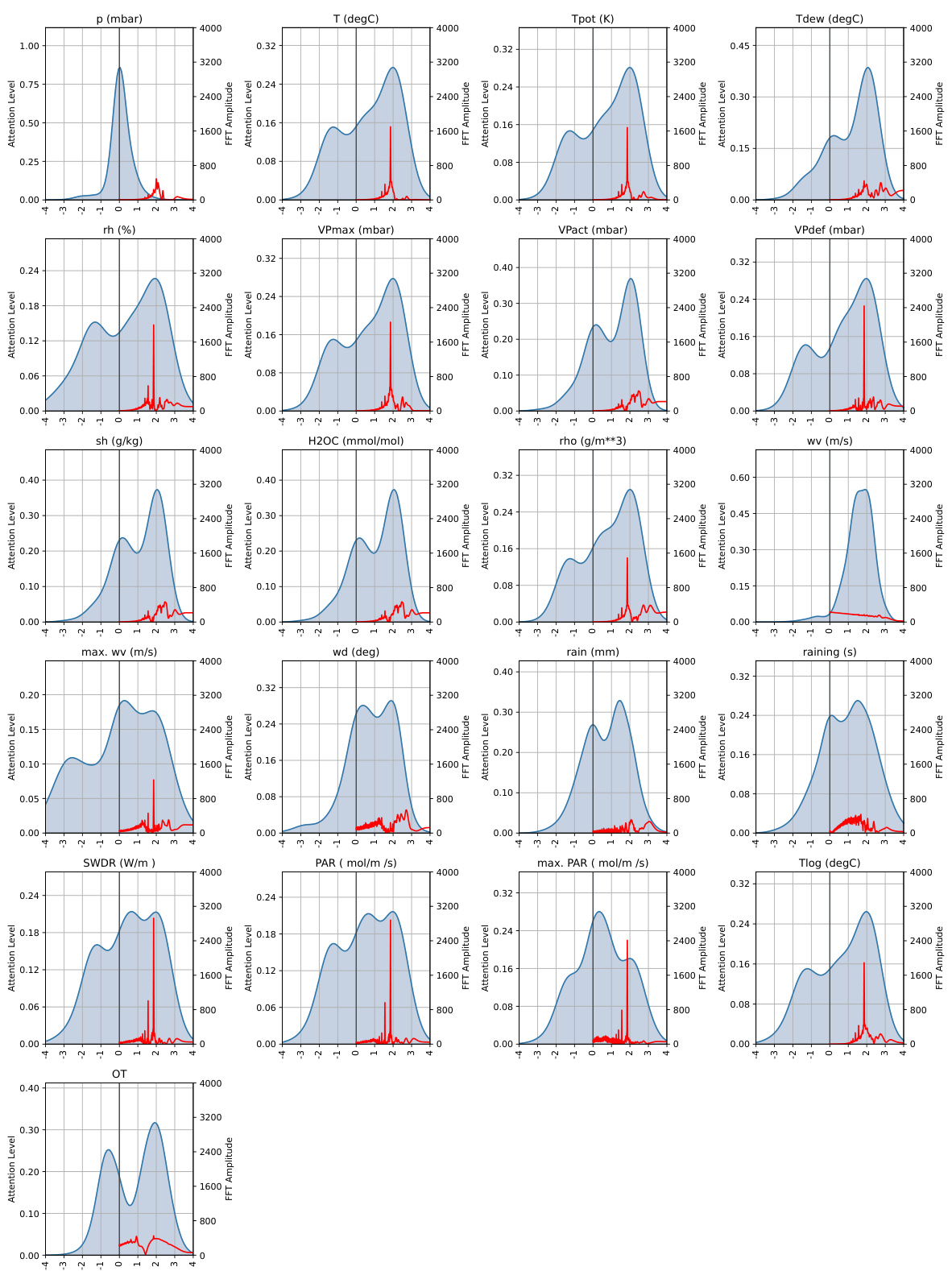
This figure shows an analysis of the Spectral Attention (SA) matrix from a DLinear model trained for a 720-step prediction task using weather and ETTh1 datasets. Panel (a) displays a heatmap of the SA matrix which shows the weights applied to different frequencies. Panels (b)-(d) show the attention applied to different frequencies and their corresponding Fast Fourier Transform (FFT) graphs, demonstrating how the model attends to various frequencies for each dataset.

This figure analyzes the SA-matrix learned by the DLinear model during training for 720-step ahead prediction on Weather and ETTh1 datasets. Panel (a) shows a heatmap of the SA-matrix, visually representing how much attention the model pays to different frequency components. Panels (b)-(d) show the attention weight distribution and frequency spectrum (FFT) of specific channels (Weather-Temperature, Weather-SWDR, and ETTh1-HULL), further illustrating the frequency components attended by the SA-matrix in each case. These visualizations aim to demonstrate how Spectral Attention effectively captures long-range trends by focusing on relevant frequency components.
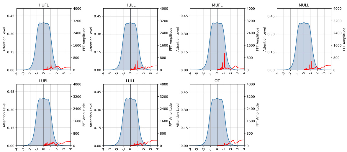
This figure shows the analysis of the SA-matrix for the DLinear model trained with a 720 prediction length on the Weather and ETTh1 datasets. The heatmap visualizes the learnable parameters of the SA-matrix, showing which frequencies the model attends to for each feature. The attention graphs and FFT graphs illustrate the correlation between the attention distribution and frequency components of the data, showing that the BSA effectively captures the long-range trend of the data.
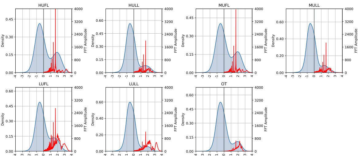
This figure shows the analysis of the SA-matrix for the DLinear model trained on a 720-step prediction task. The heatmap visualizes the learned weights in the SA-matrix, indicating which frequencies are most attended to for each feature. The other panels (b)-(d) show attention weights and corresponding FFT (Fast Fourier Transform) graphs for specific variables in the Weather and ETTh1 datasets, demonstrating the model’s attention to low-frequency components (long-term trends).
This figure provides a detailed analysis of the spectral attention (SA) matrix used in the DLinear model. The SA-matrix’s heatmap (panel a) reveals the learned weights of various frequency components for the Weather and ETTh1 datasets. Panels (b)-(d) display these learned weights alongside corresponding attention values and the Fast Fourier Transform (FFT) graphs of the raw signals. This allows for a visual comparison of learned weights with the frequency distributions found in actual data, providing insights into how effectively SA-matrix captures long-range dependencies.

This figure shows the analysis of the SA-matrix learned by the DLinear model trained on the 720-step prediction task for the Weather and ETTh1 datasets. The heatmap of the SA-matrix is shown in panel (a). The attention and FFT graphs are shown in panels (b) through (d). These graphs help to visualize how the SA-matrix focuses on low-frequency components of the data for long-range dependency modeling.
This figure illustrates the difference between conventional time series forecasting approaches and the proposed method. Panel (a) shows how time series data is sampled sequentially with high temporal correlation between consecutive samples. Panel (b) depicts conventional methods that ignore this temporal information by shuffling the data. Panel (c) presents the proposed method which preserves the temporal correlation to enable modeling long-range dependencies that go beyond the look-back window.
More on tables

This table presents the performance improvement achieved by using the Batched Spectral Attention (BSA) module compared to the baseline model. The improvements are calculated as the percentage change in MSE and MAE metrics across different input lengths (48, 96, 192) for the iTransformer model, considering the average across four prediction lengths and three random seeds. The table specifically focuses on the iTransformer model, but Appendix D.2. provides the full results for other models as well.

This table shows the percentage increase in computational cost (time, memory, and number of parameters) when using the Batched Spectral Attention (BSA) module compared to the baseline models (TimesNet, iTransformer, Crossformer, and PatchTST) on the PEMS03 dataset. The results are averaged over three random seeds and four prediction lengths. Appendix D.3 provides more detailed results for other datasets.
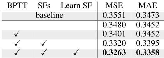
This table presents the ablation study results for the Batched Spectral Attention (BSA) module, showing the impact of its three key components: Backpropagation Through Time (BPTT), multiple smoothing factors (SFs), and learnable smoothing factors (Learn SF). Each row represents a different combination of these components, indicating whether they were enabled (✓) or disabled. The baseline represents the performance without BSA. The MSE and MAE (Mean Absolute Error) values show the model performance for each configuration, demonstrating the contribution of each component to the overall performance improvement.

This table presents the average forecasting performance results across multiple datasets and models. It compares the performance of the baseline models against those using the proposed BSA (Batched Spectral Attention) method, evaluating Mean Squared Error (MSE) and Mean Absolute Error (MAE). Statistical significance (p-value < 0.05) is indicated with red highlighting. The table also provides averages across all datasets for a broad performance comparison.
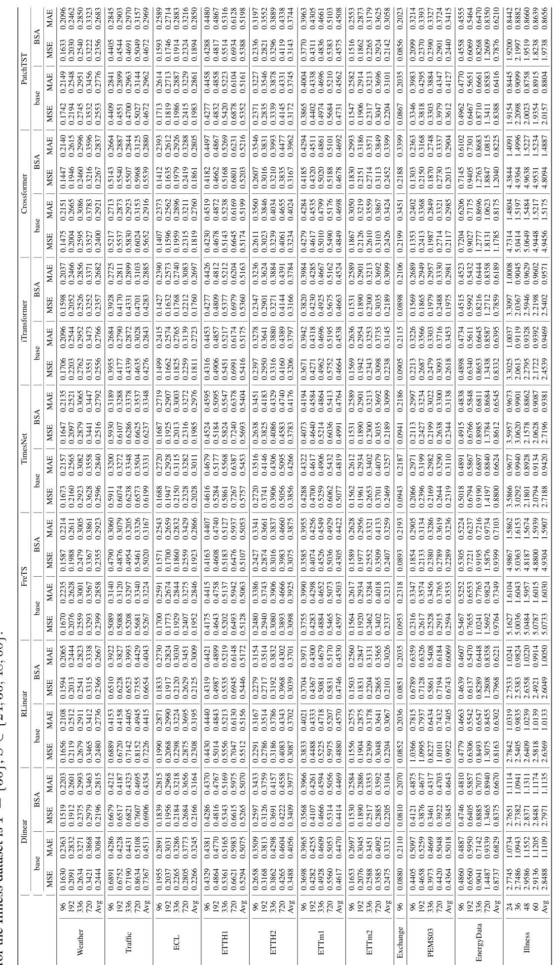
This table presents the average forecasting performance results across 11 real-world datasets and 7 forecasting models (DLinear, RLinear, FreTS, TimesNet, iTransformer, Crossformer, PatchTST) for four different prediction lengths (S = 96, 192, 336, 720). The table compares the performance of the base models with the BSA module added. It highlights the average Mean Squared Error (MSE) and Mean Absolute Error (MAE) for each model and dataset. Statistical significance (p<0.05) is indicated using red font. The average performance across all datasets is shown in the ‘Avg’ column.

This table presents the average forecasting performance results across four different prediction lengths (96, 192, 336, and 720 time steps) and three random seeds. The results are shown for eleven real-world datasets and seven forecasting models. Higher performance with BSA (Bolded) compared to the base model is highlighted, along with statistical significance (p-value < 0.05) indicated in red. Abbreviations for the datasets are provided.
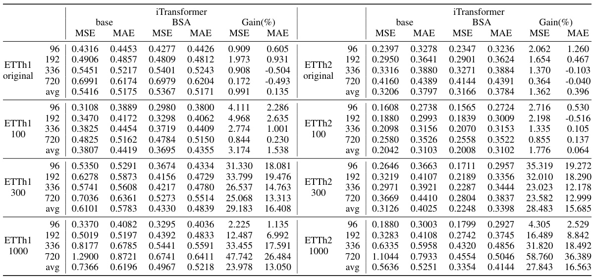
This table presents the average forecasting performance results across different prediction lengths (96, 192, 336, and 720 time steps) and three random seeds, comparing the base model and the model with the proposed BSA module. It includes results for 11 real-world datasets and seven different forecasting models, showing Mean Squared Error (MSE) and Mean Absolute Error (MAE). Statistical significance (p-value < 0.05) is indicated with red coloring. The table averages results for multiple datasets and models, with full results detailed in the appendix.

This table presents the average forecasting performance results across 11 real-world datasets and 7 forecasting models. The results are presented for four different prediction lengths (96, 192, 336, and 720 time steps) and averaged across three separate training runs to show the model’s robustness. The table highlights the Mean Squared Error (MSE) and Mean Absolute Error (MAE) for each model (base model vs. model with BSA). Bold values indicate statistically significant improvements of BSA over the base model (p<0.05). The table also provides an average performance across all datasets.
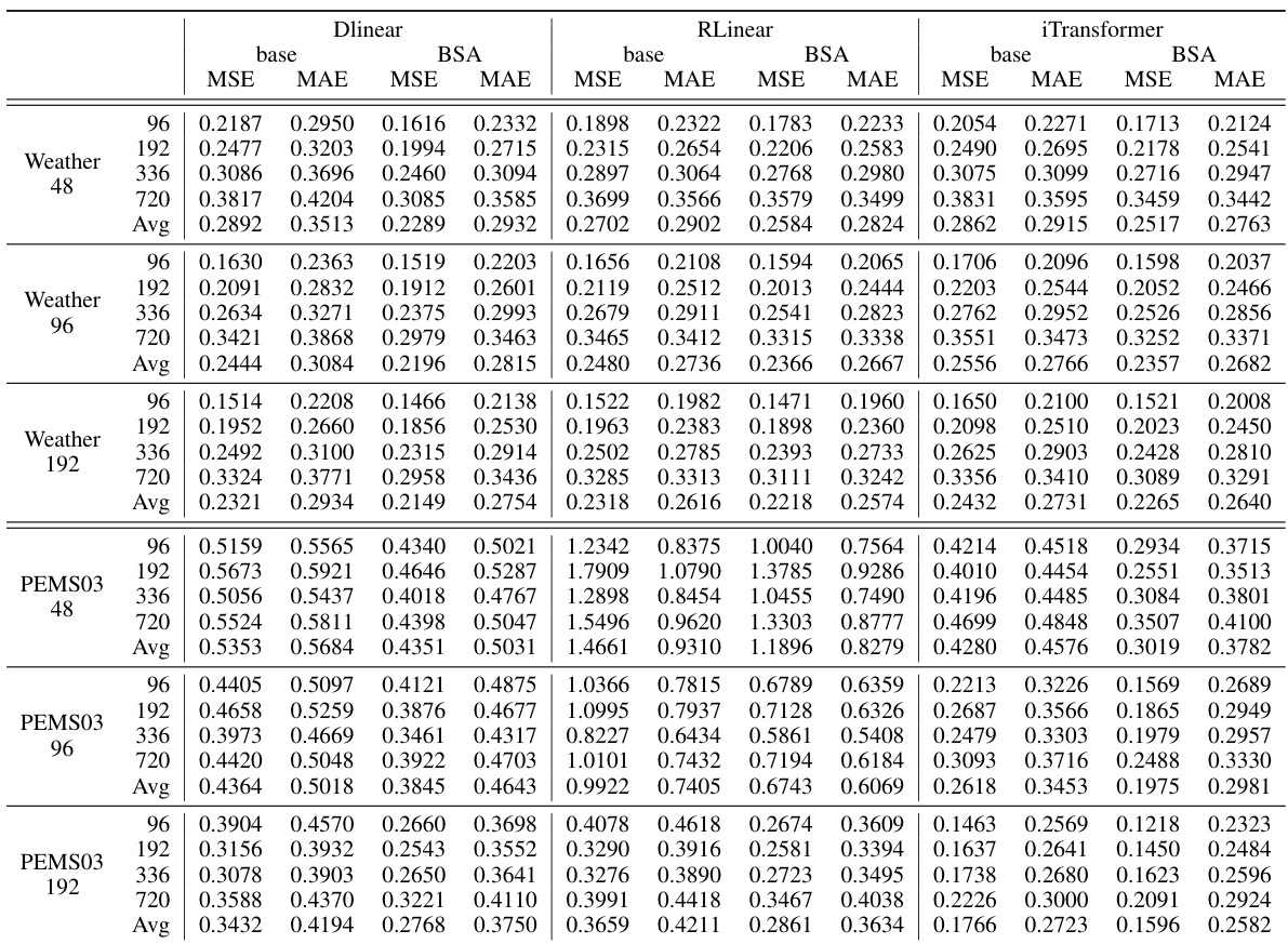
This table presents the average forecasting results across four different prediction lengths (96, 192, 336, and 720 time steps) and three random seeds for seven different forecasting models (DLinear, RLinear, FreTS, TimesNet, iTransformer, Crossformer, and PatchTST) applied to eleven real-world datasets (Weather, Traffic, ECL, ETTh1, ETTh2, ETTm1, ETTm2, Exchange, PEMS03, EnergyData, and Illness). The table shows the Mean Squared Error (MSE) and Mean Absolute Error (MAE) for each model and dataset, highlighting the improvements achieved by using the Batched Spectral Attention (BSA) mechanism. Bolded values indicate statistically significant performance gains of BSA over the baseline models (p<0.05, using a paired t-test).

This table presents the average forecasting performance results across four different prediction lengths (96, 192, 336, and 720 time steps) and three random seeds for eleven real-world datasets and seven forecasting models. The table compares the performance of the baseline models against the models enhanced with the Batched Spectral Attention (BSA) mechanism. Higher performance of BSA-enhanced models is highlighted in bold. The ‘Avg.’ column shows the average performance across all datasets, and red highlights statistically significant improvements (p<0.05) based on paired t-tests.
Full paper#
