TL;DR#
Graph data, unlike array data, poses challenges for applying the highly successful convolutional neural networks (CNNs). Existing graph neural networks (GNNs) often lack the expressiveness of CNNs. This research addresses these limitations by creating a new class of GNNs called Quantized Graph Convolutional Networks (QGCNs).
QGCNs overcome the limitations by decomposing the convolution operation into smaller, non-overlapping sub-kernels, enabling them to work with graph structures. The assignment of these sub-kernels is learnable. QGCNs are shown to match or exceed the performance of other state-of-the-art GNNs on various benchmark tasks, demonstrating their effectiveness in handling real-world graph datasets. This work provides a significant step forward in applying CNN-like architectures to analyze complex graph data.
Key Takeaways#
Why does it matter?#
This paper is crucial because it bridges the gap between Convolutional Neural Networks (CNNs) and Graph Neural Networks (GNNs). By directly extending CNNs to graphs, it offers a novel framework that leverages the strengths of CNNs while addressing challenges specific to graph data. This advance opens new avenues in various fields that deal with graph data, such as brain network modeling and social network analysis, allowing for more accurate and expressive models. It also introduces a new benchmark dataset for evaluating GNN performance.
Visual Insights#
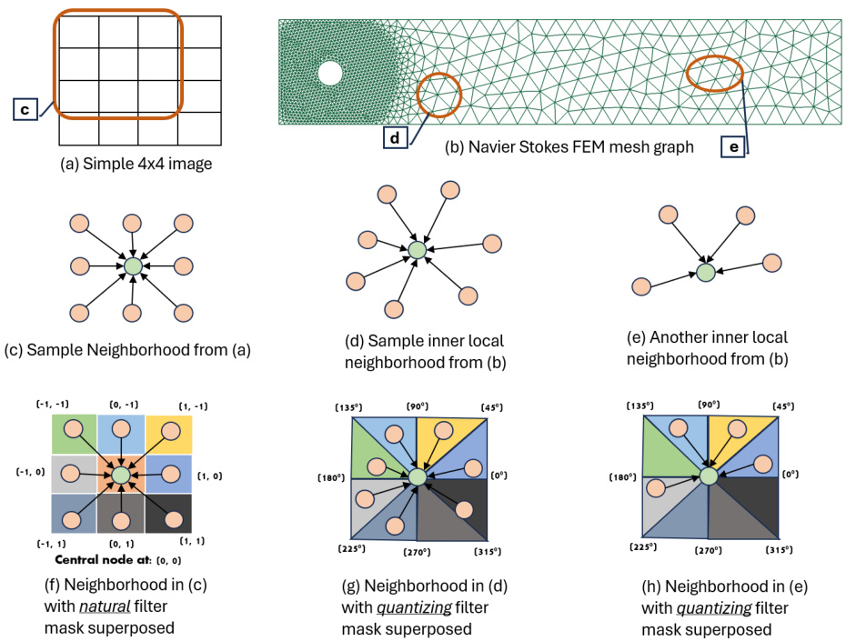
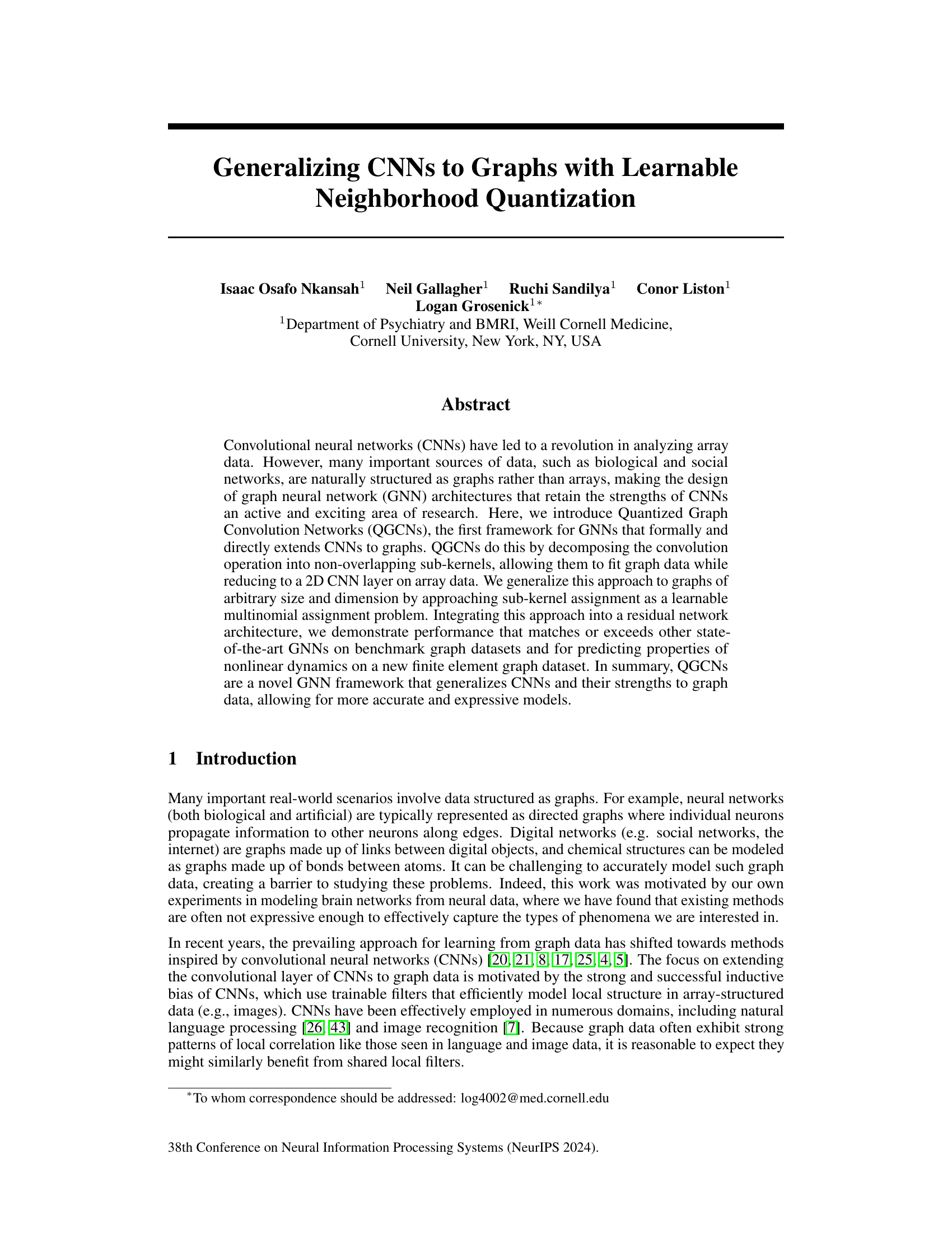
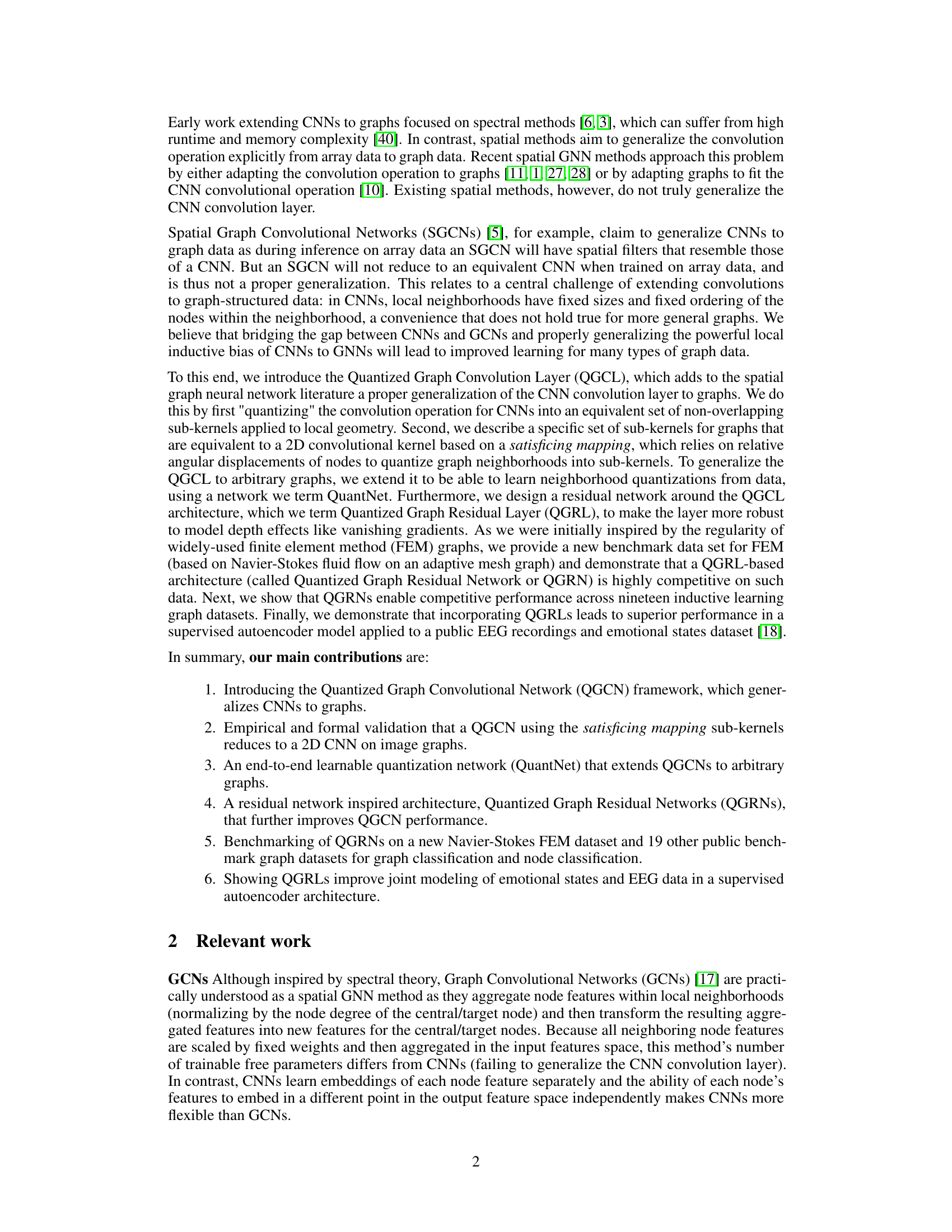
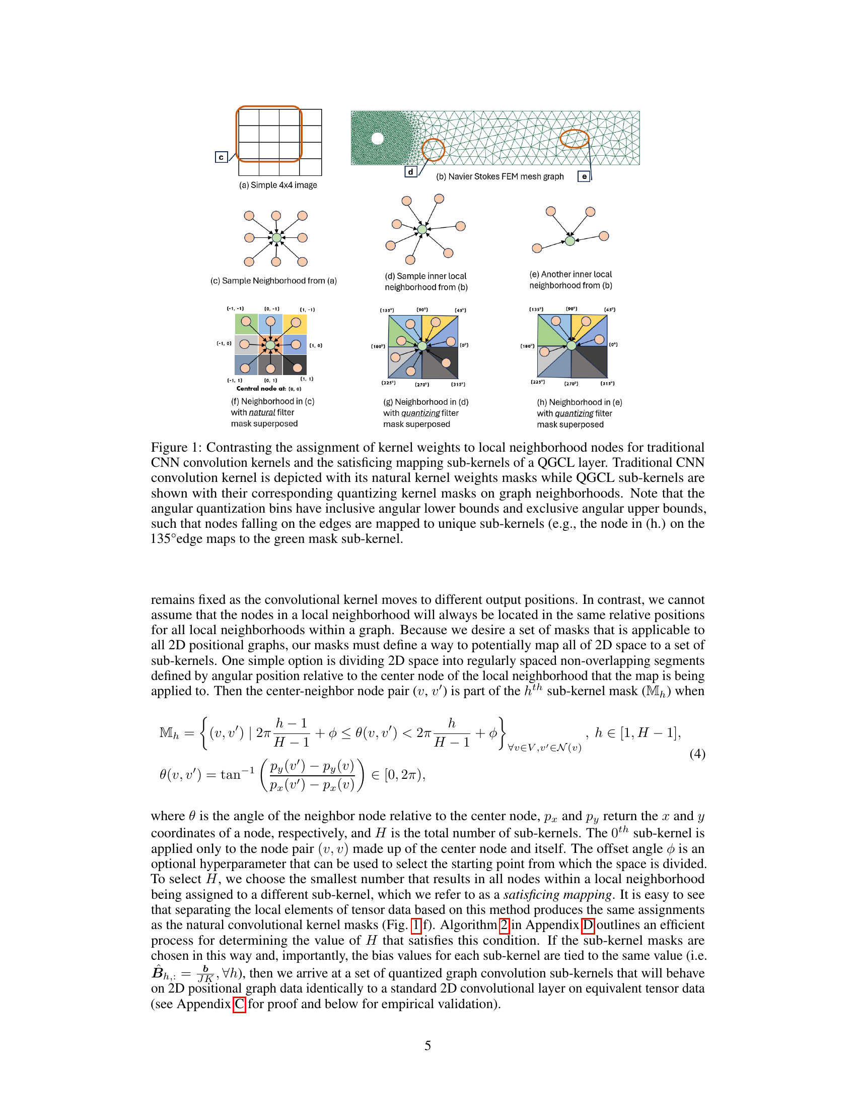
🔼 This figure compares the assignment of kernel weights in traditional CNNs and QGCNs. It illustrates how the natural convolutional masks of CNNs are mapped to sub-kernel masks in QGCNs, highlighting the differences in how neighborhood nodes are assigned to sub-kernels in both methods. The image illustrates an example of a 4x4 image graph, a Navier-Stokes FEM graph, and sample local neighborhoods from each, showing the distribution of sub-kernels.
read the caption
Figure 1: Contrasting the assignment of kernel weights to local neighborhood nodes for traditional CNN convolution kernels and the satisficing mapping sub-kernels of a QGCL layer. Traditional CNN convolution kernel is depicted with its natural kernel weights masks while QGCL sub-kernels are shown with their corresponding quantizing kernel masks on graph neighborhoods. Note that the angular quantization bins have inclusive angular lower bounds and exclusive angular upper bounds, such that nodes falling on the edges are mapped to unique sub-kernels (e.g., the node in (h.) on the 135°edge maps to the green mask sub-kernel.)
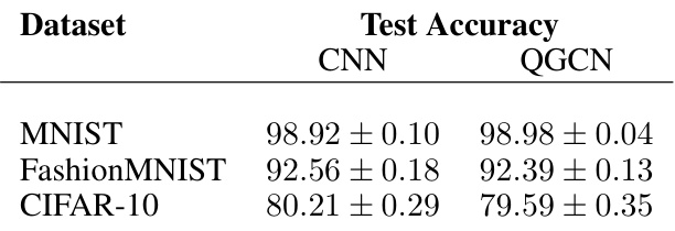
🔼 This table presents the test accuracy results for CNN and QGCN models trained on three standard image datasets: MNIST, FashionMNIST, and CIFAR-10. The results show that QGCN achieves comparable performance to CNN on these datasets, demonstrating its ability to generalize CNNs to image data.
read the caption
Table 1: Standard image datasets. CNN and QGCN model accuracies (mean ± S.D.).
In-depth insights#
CNN-to-Graph#
The concept of “CNN-to-Graph” represents a significant challenge and opportunity in machine learning. Convolutional Neural Networks (CNNs), highly successful in image processing, leverage the inherent spatial structure of image data. Adapting this strength to graph data, which lacks a fixed, regular structure, requires innovative approaches. This involves finding ways to define meaningful ’neighborhoods’ on graphs that mirror the local receptive fields of CNNs. Learnable neighborhood quantization is a promising technique to address the irregularity of graph structure. By partitioning nodes into quantized neighborhoods, this approach strives to bridge the gap between the regular grid of CNNs and the irregular topology of graphs. This allows for the use of CNN-like operations in a graph setting, potentially combining the strengths of both models. However, challenges remain in efficiently and effectively handling various graph types and sizes and maintaining the expressive power of CNN filters in a generalized graph context. Satisficing mapping and learnable quantization techniques offer paths to address these challenges, but further research is crucial in evaluating their efficacy and exploring alternative strategies.
QuantNet#
The proposed QuantNet is a crucial component of the Quantized Graph Convolutional Network (QGCN) framework, addressing the challenge of applying CNN-like convolutions to graphs with arbitrary structure. QuantNet learns a mapping from node pairs in a graph’s local neighborhood to a set of sub-kernels. This learned mapping acts as a learnable neighborhood quantization, replacing the fixed quantization scheme used when applying the QGCN framework to graphs with inherent positional information (such as images). This learnable component allows QGCN to handle complex graph structures effectively. The use of a multinomial classification approach (using an MLP) within QuantNet allows for flexibility and generalizability across different graph types. This approach contrasts with previous methods which rely on explicit positional information, making QuantNet more versatile and widely applicable.
QGRN Benchmarks#
The QGRN benchmark results showcase its strong performance across diverse graph datasets. Superior performance on datasets with positional descriptors highlights the model’s ability to leverage spatial information effectively, outperforming existing methods such as SGCNs. Competitive results on generic graph datasets demonstrate QGRN’s broad applicability. A novel FEM dataset further validates QGRN’s effectiveness in predicting properties of complex, real-world systems. The consistent high accuracy across various tasks underscores the model’s robust generalization capabilities and suggests potential for broader applications in various domains involving graph structured data. Further investigation is needed to understand the impact of different quantization strategies on model performance and to improve computational efficiency for larger graphs.
Limitations#
A thoughtful analysis of the limitations section of a research paper would delve into the methodological constraints, such as the specific datasets used and their potential biases, which might limit the generalizability of the findings. It would also examine the computational limitations, including the time and resources required to train the models, and any limitations arising from the chosen architectural decisions. Furthermore, a critical evaluation should touch upon the scope of the study, including limitations of the theoretical framework or the specific tasks addressed, acknowledging the potential need for future work to expand on the presented results. Assumptions made during the research and their impact on the conclusions are also key considerations. Finally, the analysis should discuss whether the results are sufficiently robust and the possibility of improving the model’s performance or expanding its applicability to other scenarios, emphasizing the need for thorough validation and testing to enhance the reliability of the conclusions.
Future Work#
The authors acknowledge the limitations of their current QGCN implementation, particularly regarding computational efficiency and the inability to handle all CNN configurations (odd-sized kernels or strides other than one). Future work should prioritize optimizing QGCL’s implementation through parallelization and exploring alternative quantization strategies beyond angular and learnable methods. Investigating the performance of QGCNs in deeper architectures, such as U-Nets, and applying them to more diverse inductive and transductive graph learning tasks is also crucial. Exploring the potential of different masking functions for QGCL sub-kernels would unlock further expressiveness and efficiency. This might involve adapting or designing novel mask functions tailored to specific graph characteristics or problem domains. Finally, a thorough investigation of QGCN’s sensitivity to various hyperparameters and their impact on overall performance is needed to develop a better understanding and improve the robustness of the model.
More visual insights#
More on figures

🔼 This figure shows the architecture of QuantNet and Quantized Graph Residual Layer (QGRL). QuantNet is a learnable network that dynamically quantizes nodes into subkernels within local neighborhoods. QGRL is a residual network architecture that incorporates QGCL, improving its robustness and performance.
read the caption
Figure 2: QuantNet and Quantized Graph Residual Layer (QGRL). [Left] A learnable network for dynamic quantization of nodes to subkernels in different local neighborhoods. The message passing framework in PyTorch provides the source and target nodes across all edges so QGCL doesn't have any computation overheads in defining the input tensors fed into QuantNet. The output of QuantNet is the satisficing mapping used to filter the receptive fields of the QGCL subkernels. [Right] An architectural retrofit of QGCL, incorporating 2 residual blocks: (1) outer residual block for the QGCL and (2) an inner residual block for learning features from input graph messages. The network combines all features dynamically via MLP-III to prepare the final node messages for the layer.
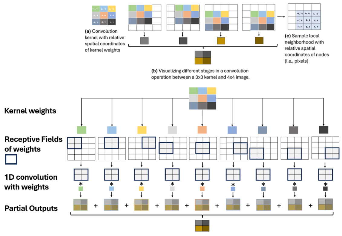
🔼 This figure demonstrates how the proposed method, Quantized Graph Convolutional Networks (QGCNs), generalizes 2D convolutional neural networks (CNNs) to graph data. Panel (a) shows a standard convolutional kernel with relative spatial coordinates of kernel weights. Panel (b) illustrates the convolution operation between a 3x3 kernel and a 4x4 image, breaking it down into steps. Panel (c) shows a sample local neighborhood on a graph with relative spatial coordinates of nodes, highlighting how the concept extends to graph data structures. Finally, the lower part of the figure shows how the 2D convolution can be decomposed into a linear combination of 1D convolutions, illustrating the connection between CNNs and QGCNs.
read the caption
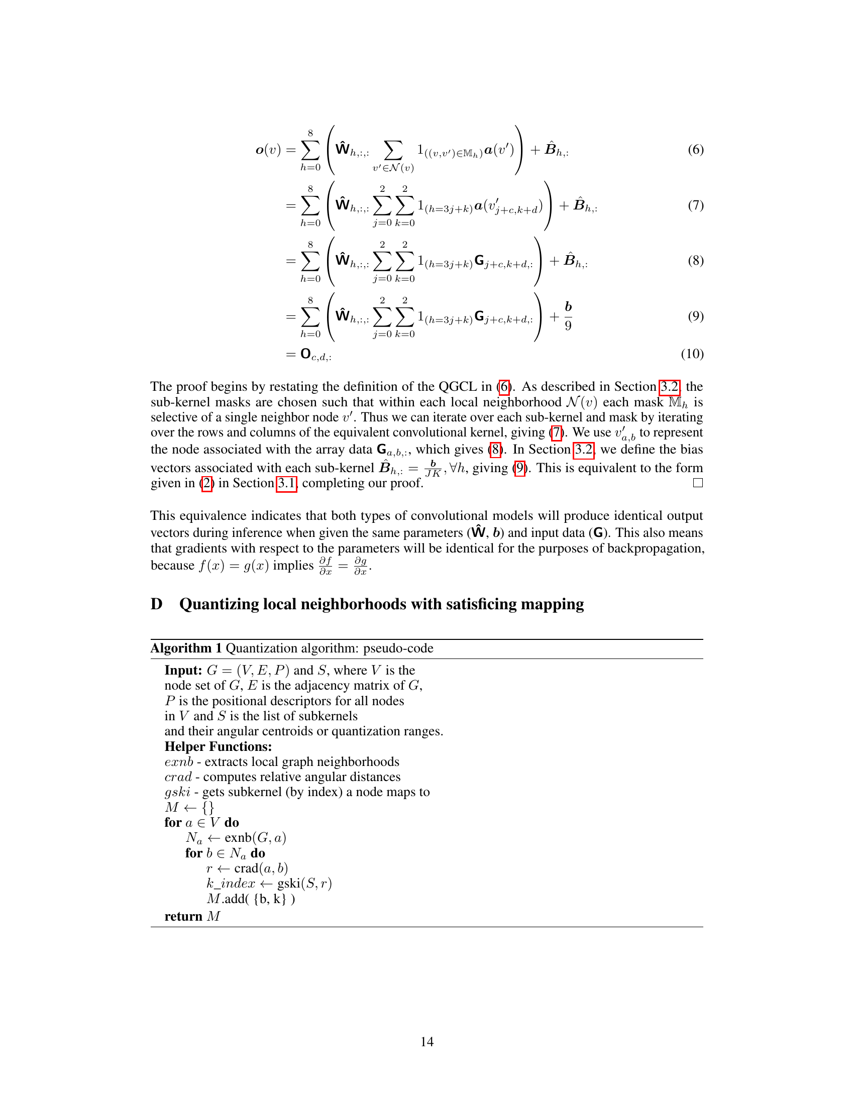
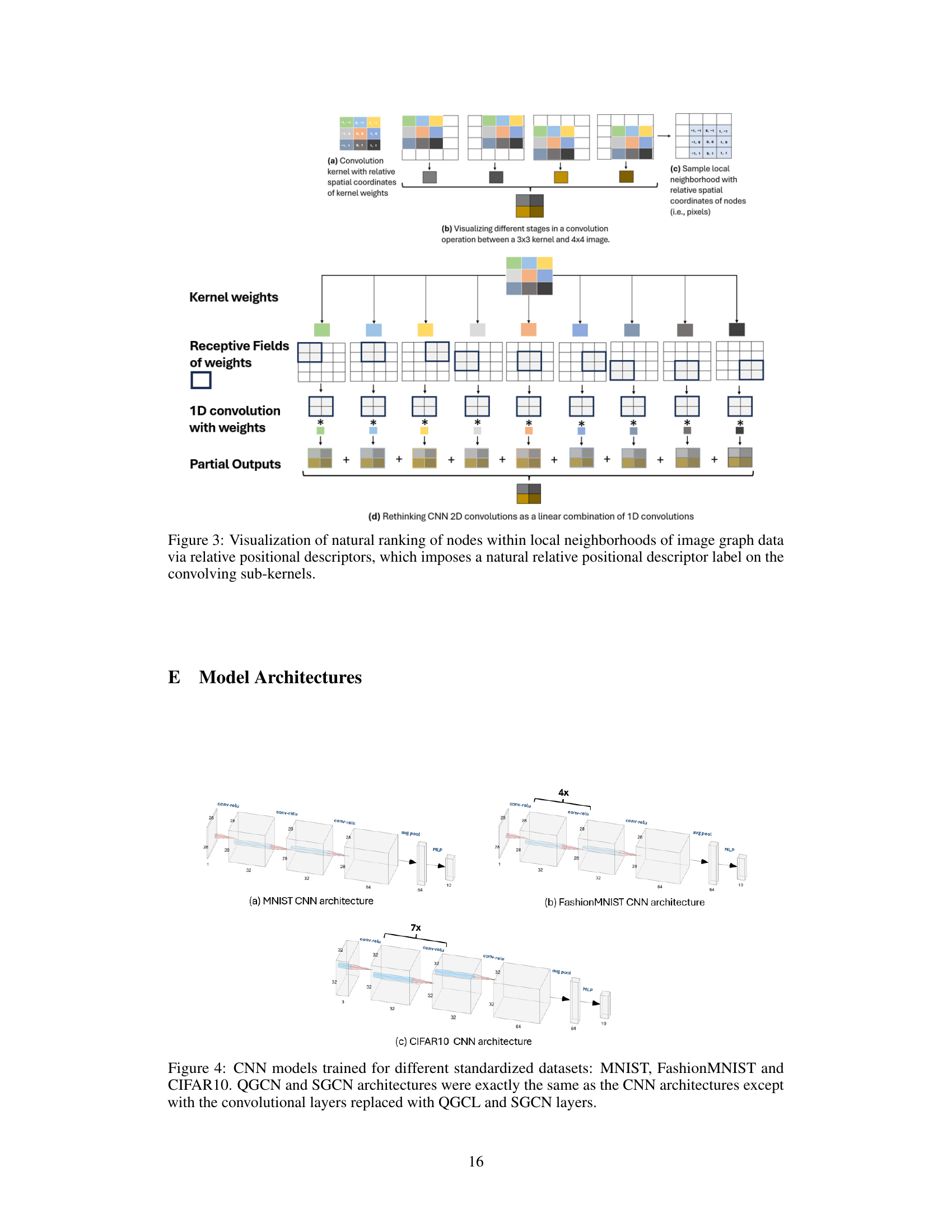
Figure 3: Visualization of natural ranking of nodes within local neighborhoods of image graph data via relative positional descriptors, which imposes a natural relative positional descriptor label on the convolving sub-kernels.

🔼 This figure demonstrates how the proposed Quantized Graph Convolutional Layer (QGCL) generalizes 2D CNN convolution to graphs. Panel (a) shows a standard 3x3 convolution kernel with the relative spatial coordinates of kernel weights highlighted. Panel (b) illustrates the convolution process, showing how the kernel slides across the image data, generating partial outputs, which are summed together to create the final output. Panel (c) demonstrates a graph representation of a local neighborhood (e.g., a small patch of pixels) with relative spatial coordinates (analogous to pixels). Panel (d) conceptually shows how a 2D convolution can be viewed as a linear combination of multiple 1D convolutions, which helps to bridge the gap between the array-based convolution of a CNN and the graph-based convolution of the QGCL. The figure highlights the use of relative positional descriptors to assign natural relative positions and descriptor labels to sub-kernels, enabling a generalization of CNN convolution to graphs.
read the caption
Figure 3: Visualization of natural ranking of nodes within local neighborhoods of image graph data via relative positional descriptors, which imposes a natural relative positional descriptor label on the convolving sub-kernels.

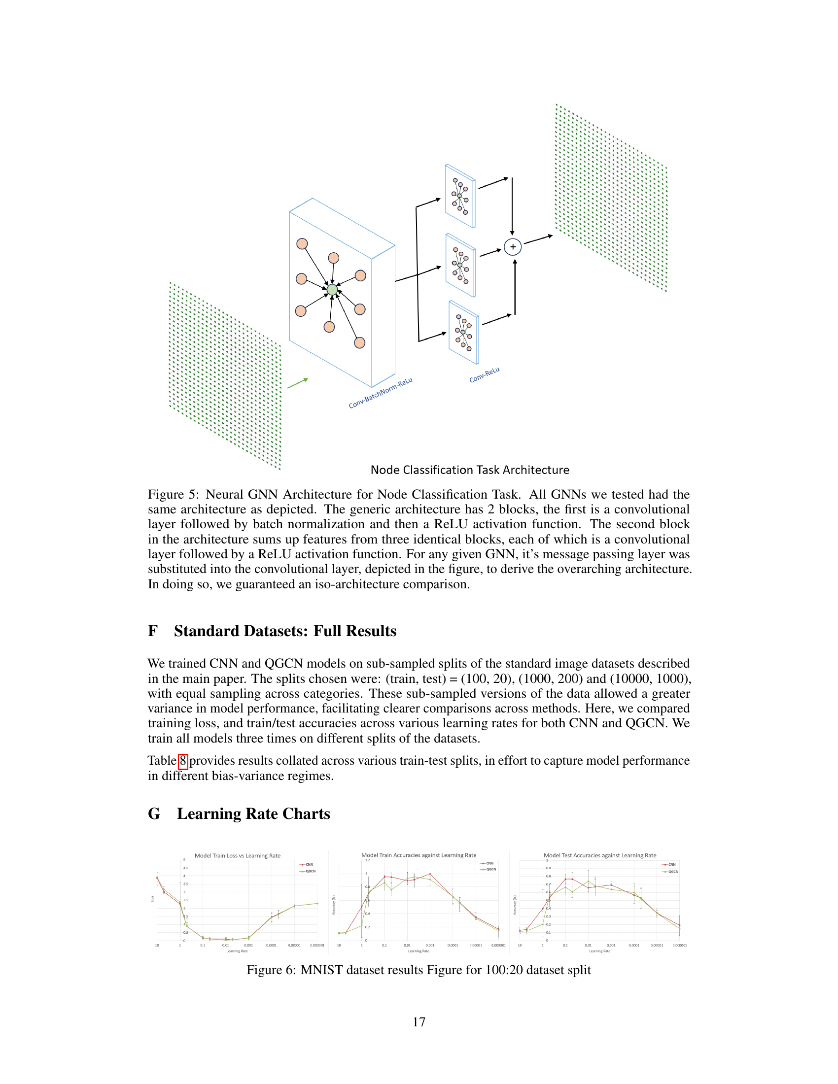
🔼 This figure shows the architecture used for node classification tasks, ensuring a fair comparison across different GNN models. The architecture consists of two main blocks: the first uses convolutional layers with batch normalization and ReLU activation, and the second sums features from three identical blocks of convolutional layers with ReLU activation. The specific message passing layer for each GNN was substituted into the convolutional layer to maintain a consistent architecture for comparison.
read the caption
Figure 5: Neural GNN Architecture for Node Classification Task. All GNNs we tested had the same architecture as depicted. The generic architecture has 2 blocks, the first is a convolutional layer followed by batch normalization and then a ReLU activation function. The second block in the architecture sums up features from three identical blocks, each of which is a convolutional layer followed by a ReLU activation function. For any given GNN, its message passing layer was substituted into the convolutional layer, depicted in the figure, to derive the overarching architecture. In doing so, we guaranteed an iso-architecture comparison.

🔼 This figure illustrates how the concept of a convolutional kernel, commonly used in CNNs for image processing, can be extended to graph data. Panel (a) shows a convolutional kernel with the relative spatial coordinates of its weights explicitly labeled. Panel (b) visually breaks down the convolution process, showing how the kernel interacts with a small portion of the input image (4x4) to compute partial outputs, which are then summed to obtain the final output. Panel (c) translates this concept to a graph, depicting a sample neighborhood (local structure in the graph) with the relative positional coordinates of its nodes. Panel (d) highlights that 2D convolutions in CNNs can be viewed as a linear combination of 1D convolutions, which is the basis for understanding how it generalizes to graphs.
read the caption
Figure 3: Visualization of natural ranking of nodes within local neighborhoods of image graph data via relative positional descriptors, which imposes a natural relative positional descriptor label on the convolving sub-kernels.

🔼 This figure demonstrates how the proposed Quantized Graph Convolutional Layer (QGCL) extends the standard convolutional layer from image data to graph data. It contrasts the assignment of kernel weights to local neighborhood nodes in a traditional CNN convolutional kernel and the QGCL’s satisficing mapping sub-kernels. It visually depicts the natural kernel weights masks of a CNN convolutional kernel and the quantizing filter masks of QGCL sub-kernels on graph neighborhoods, highlighting how QGCL handles nodes falling on the edges of angular quantization bins. The figure uses a simple 4x4 image and a Navier-Stokes FEM mesh graph as examples, illustrating how the method naturally generalizes to different graph types.
read the caption
Figure 3: Visualization of natural ranking of nodes within local neighborhoods of image graph data via relative positional descriptors, which imposes a natural relative positional descriptor label on the convolving sub-kernels.

🔼 This figure compares the assignment of kernel weights in traditional CNNs versus QGCLs. Panel (a) shows a CNN kernel with relative spatial coordinates; panel (b) visualizes the convolution operation stages; panel (c) shows a sample local neighborhood with relative spatial coordinates; panel (d) shows a 1D convolution of weights; and the last panel shows partial outputs.
read the caption
Figure 3: Visualization of natural ranking of nodes within local neighborhoods of image graph data via relative positional descriptors, which imposes a natural relative positional descriptor label on the convolving sub-kernels.

🔼 This figure illustrates how the proposed Quantized Graph Convolutional Layer (QGCL) generalizes the traditional convolutional layer of CNNs to graph data. It contrasts the assignment of kernel weights in a traditional CNN (using natural kernel weight masks) with the QGCL’s approach using quantizing filter masks. The satisficing mapping approach is highlighted, showing how local graph neighborhoods are divided into sub-kernels based on relative angular displacements of nodes. The figure emphasizes that this approach reduces to the standard 2D CNN convolution when applied to image data represented as a graph.
read the caption
Figure 3: Visualization of natural ranking of nodes within local neighborhoods of image graph data via relative positional descriptors, which imposes a natural relative positional descriptor label on the convolving sub-kernels.

🔼 This figure contrasts the assignment of kernel weights in traditional CNNs versus the QGCL (Quantized Graph Convolutional Layer). Panel (a) shows a 3x3 convolutional kernel with weights and relative spatial coordinates. Panel (b) visualizes a convolution operation: how the kernel weights are applied to a 4x4 image, yielding partial and final outputs. Panel (c) depicts a graph representation of a local image neighborhood with relative spatial coordinates of nodes. Panel (d) reinterprets a 2D convolution as a combination of multiple 1D convolutions. This highlights how the QGCL uses relative positional information to generalize the CNN convolution to graphs, even when the spatial arrangement of nodes is irregular, as opposed to the fixed order in array data.
read the caption
Figure 3: Visualization of natural ranking of nodes within local neighborhoods of image graph data via relative positional descriptors, which imposes a natural relative positional descriptor label on the convolving sub-kernels.

🔼 This figure illustrates how the proposed Quantized Graph Convolutional Layer (QGCL) generalizes the 2D convolution operation from array data to graph data. It contrasts the assignment of kernel weights to nodes in local neighborhoods for traditional CNN convolution kernels and the satisficing mapping sub-kernels of QGCL. It shows that the QGCL uses relative positional descriptors to rank nodes within their neighborhoods, which leads to a more natural generalization of CNNs to graphs.
read the caption
Figure 3: Visualization of natural ranking of nodes within local neighborhoods of image graph data via relative positional descriptors, which imposes a natural relative positional descriptor label on the convolving sub-kernels.

🔼 This figure illustrates how the proposed Quantized Graph Convolutional Network (QGCN) generalizes the CNN convolution to graph data. It contrasts the assignment of kernel weights in traditional CNNs with the QGCN’s approach. Panel (a) shows a standard 3x3 convolutional kernel with weights and their relative positions. Panel (b) visually represents how the kernel operates on a 4x4 image; the kernel weights are applied to the overlapping receptive fields to produce a single output value for each output pixel position. Panel (c) shows how this concept is extended to graph data. The nodes within a local neighborhood are assigned sub-kernel masks, similar to how kernel weights are assigned to pixels in an image. Panel (d) further clarifies that a 2D convolution can be viewed as a linear combination of 1D convolutions.
read the caption
Figure 3: Visualization of natural ranking of nodes within local neighborhoods of image graph data via relative positional descriptors, which imposes a natural relative positional descriptor label on the convolving sub-kernels.

🔼 This figure compares the assignment of kernel weights to local neighborhood nodes for traditional CNN convolution kernels and the satisficing mapping sub-kernels of a QGCL layer. Panel (a) shows a standard convolutional kernel, (b) illustrates the convolution operation, (c) shows a sample neighborhood from a 4x4 image, (d) depicts a 1D convolution operation, (e) shows sample local neighborhoods of graph data, (f) shows a neighborhood with natural filter mask superposed, (g) and (h) show neighborhoods with quantizing filter masks superposed. The figure highlights how the proposed method quantizes graph neighborhoods into sub-kernels using relative angular displacements of nodes.
read the caption
Figure 3: Visualization of natural ranking of nodes within local neighborhoods of image graph data via relative positional descriptors, which imposes a natural relative positional descriptor label on the convolving sub-kernels.

🔼 This figure contrasts the assignment of kernel weights to local neighborhood nodes for traditional CNN convolution kernels and the satisficing mapping sub-kernels of a QGCL layer. It visually demonstrates how traditional CNNs use fixed-size, regularly ordered neighborhoods (like pixels in an image), while QGCLs adapt this to graphs by using a ‘satisficing mapping’ to quantize graph neighborhoods into sub-kernels based on relative angular positions of nodes. This allows QGCLs to generalize CNN convolution to graphs.
read the caption
Figure 3: Visualization of natural ranking of nodes within local neighborhoods of image graph data via relative positional descriptors, which imposes a natural relative positional descriptor label on the convolving sub-kernels.

🔼 This figure compares how traditional CNNs and QGCLs assign kernel weights to local neighborhood nodes. It highlights the difference in how the methods handle neighborhoods with varying node positions and shows how QGCLs use angular quantization to map nodes to sub-kernels, improving generalization to graphs.
read the caption
Figure 1: Contrasting the assignment of kernel weights to local neighborhood nodes for traditional CNN convolution kernels and the satisficing mapping sub-kernels of a QGCL layer. Traditional CNN convolution kernel is depicted with its natural kernel weights masks while QGCL sub-kernels are shown with their corresponding quantizing kernel masks on graph neighborhoods. Note that the angular quantization bins have inclusive angular lower bounds and exclusive angular upper bounds, such that nodes falling on the edges are mapped to unique sub-kernels (e.g., the node in (h.) on the 135°edge maps to the green mask sub-kernel.)

🔼 This figure compares the assignment of kernel weights in traditional CNNs and QGCNs. It highlights how CNNs use fixed kernel weights for local neighborhoods with fixed ordering, while QGCNs use learnable sub-kernels that are more flexible for graphs with irregular structures. The satisficing mapping approach divides the local graph neighborhood into sub-kernels based on the angle of nodes relative to the center node. This allows for consistent mapping across diverse graphs.
read the caption
Figure 1: Contrasting the assignment of kernel weights to local neighborhood nodes for traditional CNN convolution kernels and the satisficing mapping sub-kernels of a QGCL layer. Traditional CNN convolution kernel is depicted with its natural kernel weights masks while QGCL sub-kernels are shown with their corresponding quantizing kernel masks on graph neighborhoods. Note that the angular quantization bins have inclusive angular lower bounds and exclusive angular upper bounds, such that nodes falling on the edges are mapped to unique sub-kernels (e.g., the node in (h.) on the 135°edge maps to the green mask sub-kernel.)
More on tables

🔼 This table compares the performance of QGRN and SGCN models on several custom graph datasets. The datasets include binary and denary classification tasks based on simulated Navier-Stokes fluid flow, along with established graph datasets like AIDS and Letter. For each dataset, the table shows the number of model parameters (k), floating-point operations (FLOPs), and test accuracy. This provides a quantitative comparison of the two methods across different graph types and complexities.
read the caption
Table 2: Custom Graph Datasets. QGRN and SGCN Performance Comparison
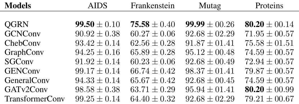
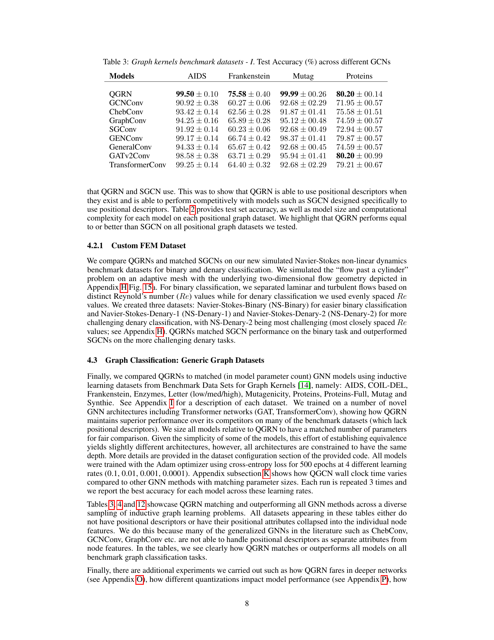
🔼 This table presents the test accuracy results of various Graph Convolutional Networks (GCNs) on four benchmark graph datasets: AIDS, Frankenstein, Mutag, and Proteins. The models compared include QGRN, GCNConv, ChebConv, GraphConv, SGConv, GENConv, GeneralConv, GATv2Conv, and TransformerConv. The table shows the mean test accuracy and standard deviation for each model on each dataset, allowing for a comparison of the performance of different GCN architectures on these common benchmark tasks.
read the caption
Table 3: Graph kernels benchmark datasets - I. Test Accuracy (%) across different GCNS

🔼 This table presents a comparison of the performance of various Graph Convolutional Networks (GCNs) on several benchmark datasets from the Benchmark Data Sets for Graph Kernels collection. The datasets represent various graph characteristics and complexities. The table shows the test accuracy achieved by each GCN model on each dataset, providing insights into their relative performance across different graph structures and properties.
read the caption
Table 4: Graph kernels benchmark datasets - II. Test Accuracy (%) across different GCNs

🔼 This table presents the results of node classification experiments on homophilic datasets. It compares the performance of several Graph Convolutional Network (GCN) models, including QGRN (the model proposed in the paper), against various benchmark datasets. The results are expressed as the test accuracy (percentage), which measures the percentage of correctly classified nodes in the test set for each model and dataset. The table shows the mean and standard deviation of the test accuracy across multiple trials.
read the caption
Table 18: Homophilic node classification datasets. Test Accuracy (%) across different GCNs

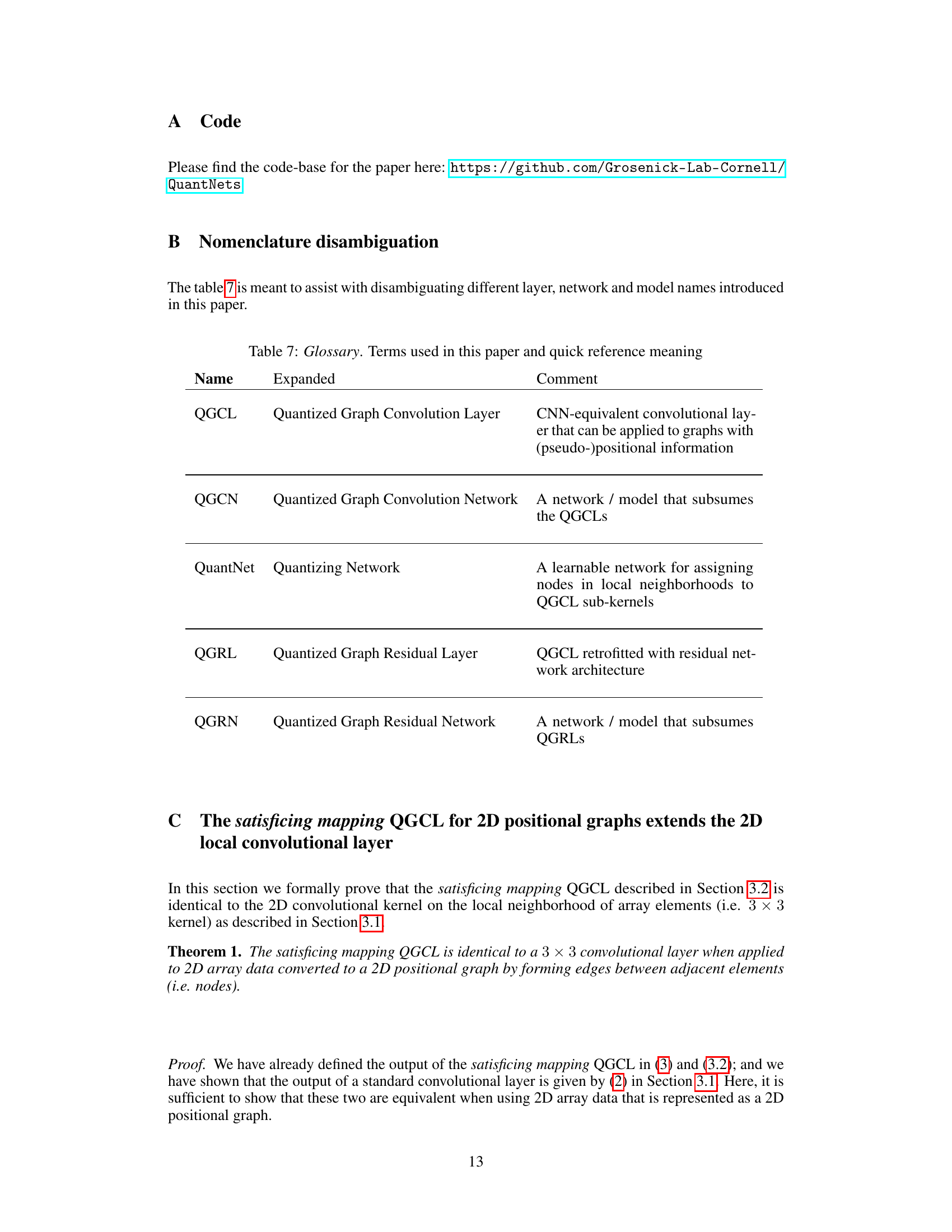
🔼 This table presents the results of a supervised autoencoder model applied to EEG data. The model used QGRN and SGCN architectures to predict emotional valence (positive or negative) from EEG data. The table shows the mean and standard error of the mean (SEM) for three metrics across all subjects: Mean Squared Error (MSE) loss for the generative part of the model, cross-entropy (CE) loss for the supervised classification part, and Area Under the Curve (AUC) of the ROC curve. The results indicate that the QGRN-based model outperforms the SGCN-based model in all three metrics.
read the caption
Table 6: EEG SAE test set performance. All values are presented as the mean±SEM over all subjects.
🔼 This table presents a comparison of the test accuracy achieved by Convolutional Neural Networks (CNNs) and Quantized Graph Convolution Networks (QGCNs) on three standard image datasets: MNIST, Fashion-MNIST, and CIFAR-10. The results show the mean and standard deviation of the test accuracy across multiple trials, demonstrating the equivalence in performance between the two models on this type of data.
read the caption
Table 1: Standard image datasets. CNN and QGCN model accuracies (mean ± S.D.)

🔼 This table presents the results of comparing the performance of Convolutional Neural Networks (CNNs) and Quantized Graph Convolutional Networks (QGCNs) on three standard image datasets: MNIST, Fashion-MNIST, and CIFAR-10. The table shows the mean and standard deviation of the test accuracy for each model on each dataset. The results demonstrate the nearly identical performance of CNNs and QGCNs on image data, supporting the claim that QGCNs are a generalization of CNNs.
read the caption
Table 1: Standard image datasets. CNN and QGCN model accuracies (mean ± S.D.).

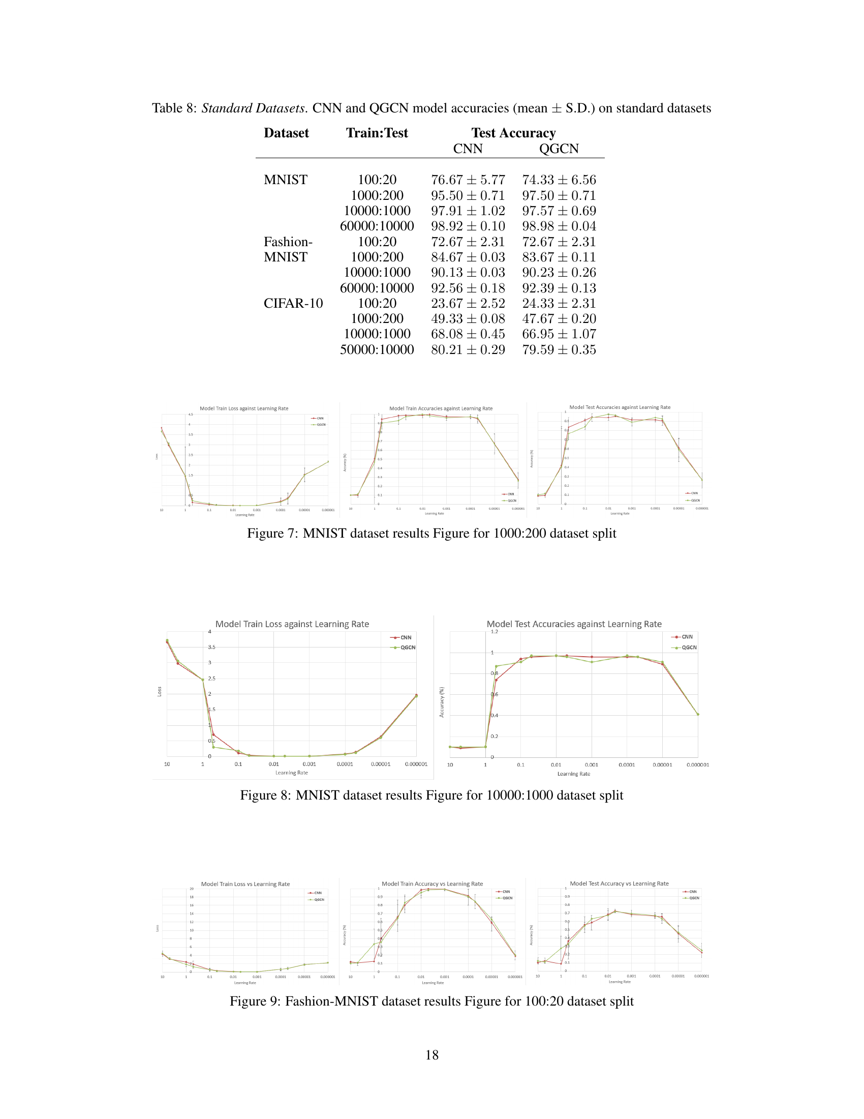
🔼 This table presents the results of training CNN and QGCN models on different sized subsets of the MNIST, Fashion-MNIST, and CIFAR-10 datasets. The purpose is to show the equivalence of CNN and QGCN models across various train-test split ratios, demonstrating consistent performance and mitigating dataset ceiling effects that could skew results when training on the full dataset.
read the caption
Table 8: Standard Datasets. CNN and QGCN model accuracies (mean ± S.D.) on standard datasets

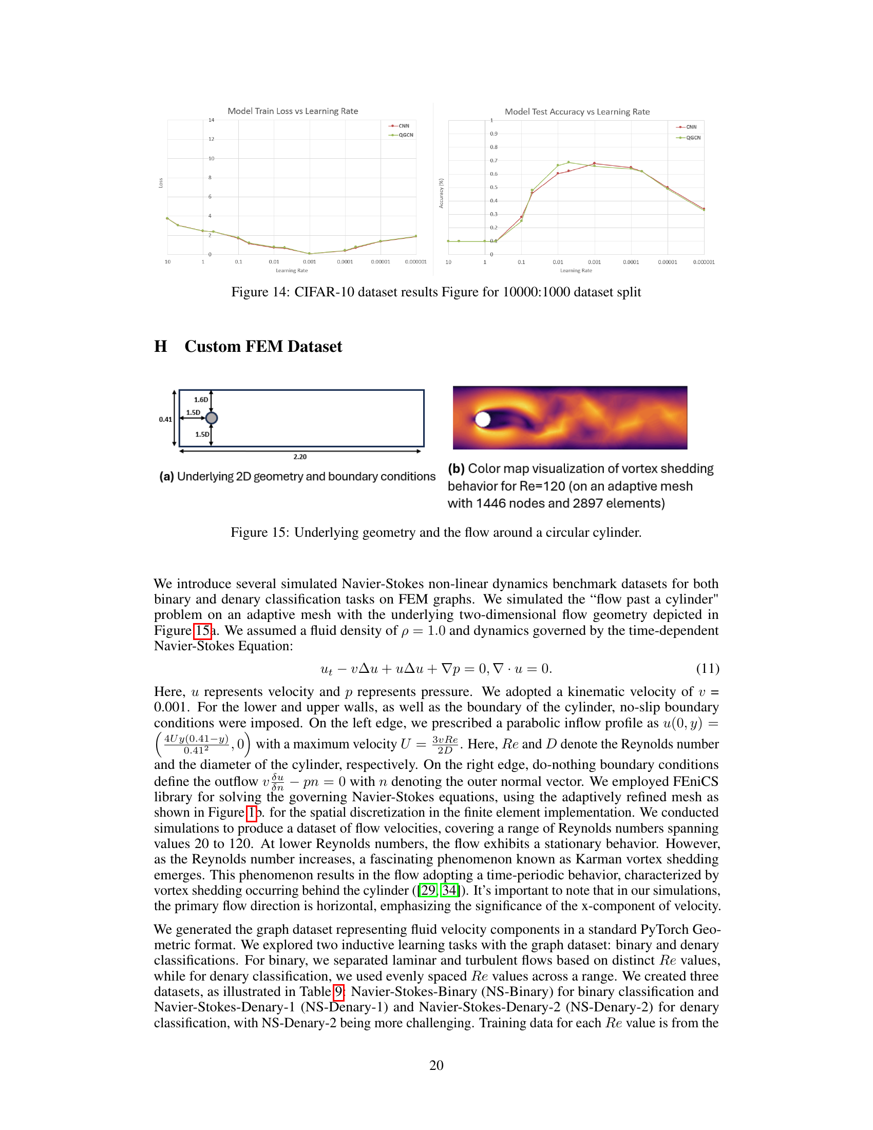
🔼 This table shows the range of Reynolds numbers (Re) used for generating the three custom Navier-Stokes datasets (NS-Binary, NS-Denary-1, and NS-Denary-2). The Re range and step-size are specified for each dataset. The binary classification dataset, NS-Binary, uses a laminar flow range (20-40) and a turbulent flow range (100-120). The denary datasets use a wider range of Re values with different step sizes.
read the caption
Table 9: The table captures the different Re ranges we considered for the different custom datasets and the step sizes. Notice in the binary case that Re = 20-40 are grouped in laminar class and 100-120 into the turbulent flow class.

🔼 This table presents different train-test splits used for the custom FEM datasets (NS-Binary, NS-Denary-1, NS-Denary-2) along with the corresponding training time periods in seconds. It shows how the amount of training data affects the model’s performance. The different splits provide variations in the bias-variance tradeoff during model training and evaluation.
read the caption
Table 10: Shown in the table are different custom dataset splits we have provided as part of this paper. The third column captures the training time period per Re from which train data were aggregated from the FEM time series solutions

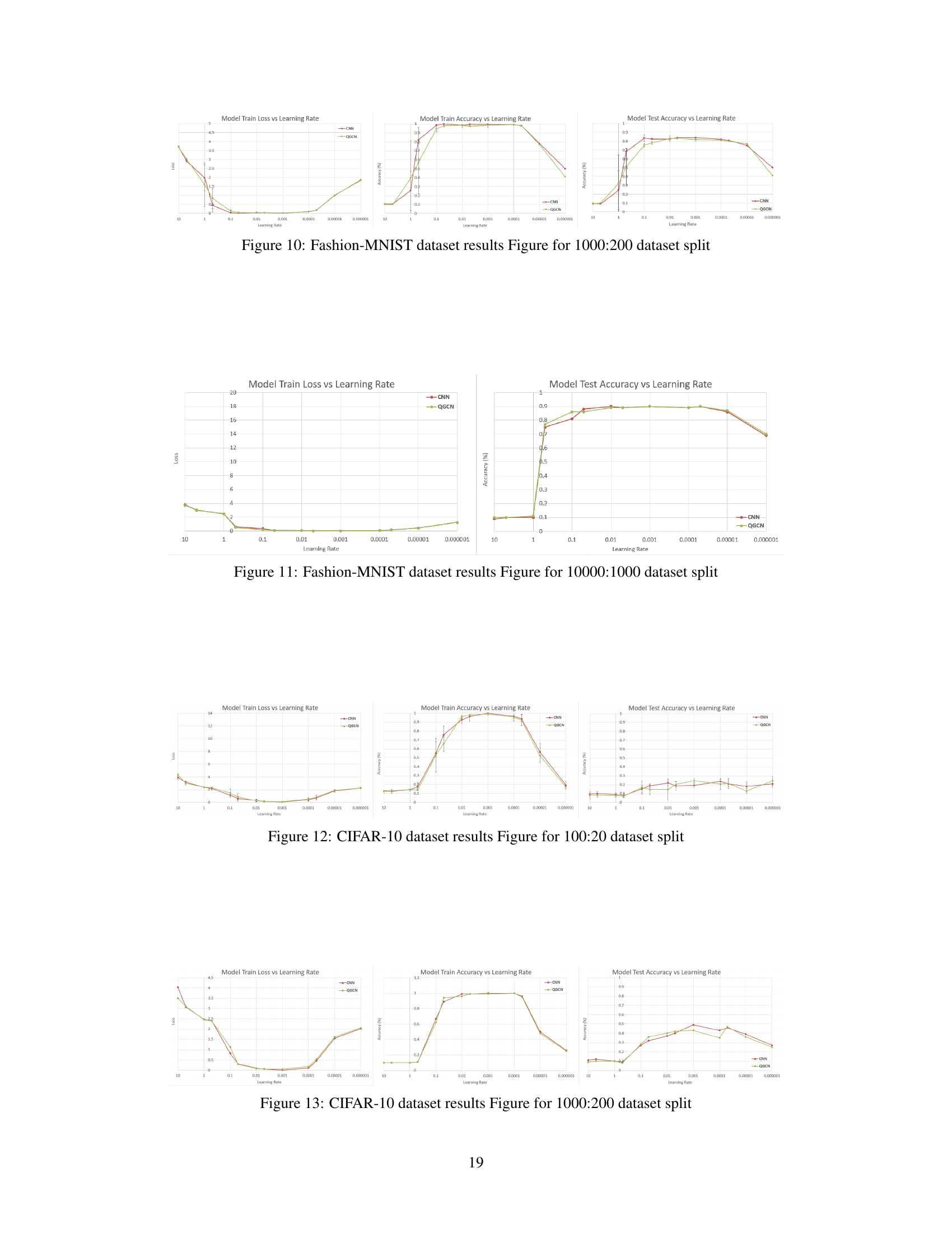
🔼 This table presents the results of training CNN and QGCN models on various subsets of three standard image datasets: MNIST, Fashion-MNIST, and CIFAR-10. Different train-test splits are used (100:20, 1000:200, 10000:1000, and 60000:10000) to explore the impact of dataset size on model performance. The table shows the mean and standard deviation of test accuracy for both CNN and QGCN models on each dataset and split.
read the caption
Table 8: Standard Datasets. CNN and QGCN model accuracies (mean ± S.D.) on standard datasets

🔼 This table presents a comparison of the test accuracy achieved by various Graph Convolutional Networks (GCNs) on four different graph kernel benchmark datasets: AIDS, Frankenstein, Mutag, and Proteins. The results show the mean test accuracy and standard deviation for each GCN model on each dataset, allowing for a direct comparison of model performance across different datasets and GCN architectures.
read the caption
Table 3: Graph kernels benchmark datasets - I. Test Accuracy (%) across different GCNs

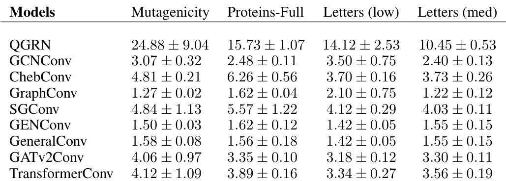
🔼 This table presents a comparison of model sizes (number of parameters) across different Graph Convolutional Network (GCN) models for various graph kernel benchmark datasets. The datasets include AIDS, Frankenstein, Mutag, Mutagenicity, Proteins, and Proteins-Full. The table helps illustrate the relative complexity of each model architecture.
read the caption
Table 13: Graph kernels benchmark datasets - I. Model sizes (number of parameters)

🔼 This table presents the number of parameters (model size) for different Graph Convolutional Network (GCN) models across six benchmark datasets from the Graph Kernels benchmark datasets. The datasets include Synthie, Letters (high, low, medium), Enzymes, and Coil-Del. The table helps in comparing the model complexity of various GCN architectures, which is important for understanding their computational cost and potential performance differences.
read the caption
Table 14: Graph kernels benchmark datasets - I. Model sizes (number of parameters)

🔼 This table presents the Google TPU inference latency, measured in milliseconds, for various graph convolutional neural network (GCN) models on the AIDS, Frankenstein, Mutag, and Proteins datasets from the Graph Kernels benchmark. The table shows the mean and standard deviation of the latency for each model across multiple trials. It provides insights into the computational efficiency of different GCN architectures.
read the caption
Table 15: Graph kernels benchmark datasets - I. Google TPU Inference latency. Wall clock (in ms)

🔼 This table presents the number of parameters (model size) for different Graph Convolutional Network (GCN) models on four graph kernel benchmark datasets: Synthie, Letters (high), Letters (low), Letters (medium), Enzymes, and Coil-Del. It provides a comparison of model complexity across various GCN architectures.
read the caption
Table 14: Graph kernels benchmark datasets - I. Model sizes (number of parameters)
🔼 This table compares the performance of QGRN against other state-of-the-art Graph Convolutional Networks (GCNs) on several benchmark datasets from the Graph Kernels benchmark collection. The datasets represent various graph classification tasks with different characteristics, including binary and multi-class problems. The table shows the test accuracy of each model, highlighting the comparative performance of QGRN.
read the caption
Table 12: Graph kernels benchmark datasets - III. Test Accuracy (%) across different GCNs

🔼 This table presents the test accuracy results for various graph convolutional networks (GCNs) on homophilic node classification datasets. Homophilic datasets are those where nodes with similar features tend to be connected. The table compares the performance of QGRN against other GCN models such as GraphConv, GENConv, GeneralConv, and EGConv. The results show the average test accuracy and standard deviation for each model on each dataset.
read the caption
Table 18: Homophilic node classification datasets. Test Accuracy (%) across different GCNs
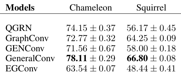
🔼 This table presents the test accuracy results for various graph convolutional network (GCN) models on heterophilic node classification datasets. Heterophilic graphs are characterized by nodes having dissimilar neighbors. The table compares the performance of QGRN against other state-of-the-art GCN models like GraphConv, GENConv, GeneralConv, and EGConv on two specific heterophilic datasets: Chameleon and Squirrel. The results show the mean test accuracy and standard deviation for each model on each dataset.
read the caption
Table 19: Heterophilic node classification datasets. Test Accuracy (%) across different GCNs

🔼 This table presents a comparison of the performance of the Quantized Graph Residual Network (QGRN) and the Spatial Graph Convolutional Network (SGCN) models on several custom graph datasets. The table includes the number of parameters (k) and FLOPS (millions) for each model, as well as the test accuracy (%) achieved on each dataset. The datasets were created by simulating nonlinear dynamics and include several variants with differing complexities.
read the caption
Table 2: Custom Graph Datasets. QGRN and SGCN Performance Comparison
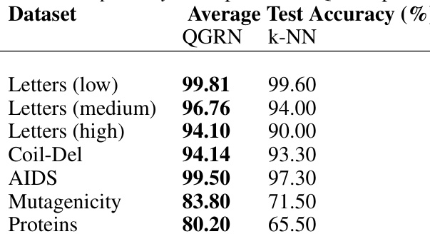
🔼 This table compares the average test accuracy of the QGRN model and a k-NN classifier on several datasets from the IAM Graph Database Repository. The datasets include variations of letter recognition tasks (with varying levels of distortion) and chemical compound and protein classification.
read the caption
Table 21: IAM Graph Database Repository. Comparison of QGRN performance to k-NN classifier
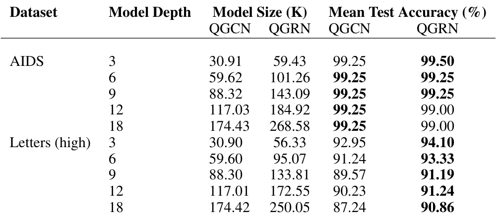
🔼 This table shows the results of training deeper QGCN and QGRN models on two datasets: AIDS and Letters (high). The AIDS dataset is a smaller, simpler binary classification problem. Letters (high) is a more complex task with 15 classes. The table shows the model depth, the model size (in thousands of parameters), and the mean test accuracy for both QGCN and QGRN models at each depth.
read the caption
Table 22: Deeper QGCN and QGRN networks. Sample results illustrating impact of deeper network on model performance

🔼 This table presents a comparison of the performance of deeper networks using two different quantization methods: satisficing mapping (SM) and QuantNet. It shows the model size and mean test accuracy for different depths (3, 6, 9, 12, and 18 layers) on two datasets: AIDS (a binary classification task) and Letters (high) (a multi-class classification task). The results illustrate how the choice of quantization method and network depth impact model performance.
read the caption
Table 23: Deeper satisficing mapping (SM) and QuantNet networks. Sample results illustrating impact of deeper network on model performance

🔼 This table compares the average test accuracy of a 3-layer QGRN model trained on several datasets, with and without using positional descriptors as input features. The results show the impact of including positional information on the model’s performance for different datasets.
read the caption
Table 24: 3-layer QGRN model analysis. Sample results for QGRN model trained with and without positional descriptors.

🔼 This table presents the results of a hyperparameter search to find the optimal number of bins (or subkernels) for the QGRN model. The search was conducted on five different graph datasets from the TUDatasets benchmark (AIDS, Enzymes, Coil-Del, Letters (high), and Proteins). For each dataset, the average test accuracy is shown for different numbers of bins (2, 3, 5, 7, and 9). The table helps to illustrate the impact of the number of bins on model performance and suggests an optimal range for this hyperparameter.
read the caption
Table 25: Number of bins - hyper-parameter search. Hyper-parameter search of optimal number of bins/subkernels for QGRN

🔼 This table presents a comparison of the test accuracy achieved by CNN and QGCN models on various standard image datasets (MNIST, Fashion-MNIST, CIFAR-10). The results are shown for different train-test split ratios to demonstrate the model’s performance across various data sizes and bias-variance trade-offs.
read the caption
Table 8: Standard Datasets. CNN and QGCN model accuracies (mean ± S.D.) on standard datasets
Full paper#
