↗ OpenReview ↗ NeurIPS Homepage ↗ Chat
TL;DR#
Machine learning models often suffer from bias, leading to unfair or discriminatory outcomes. Existing bias mitigation techniques frequently compromise accuracy. This necessitates robust solutions that balance fairness and accuracy effectively. Current methods often use Lagrangian optimization, which might overlook the complex interplay between accuracy and fairness objectives.
FairBiNN tackles this challenge using a novel bilevel optimization approach. This method models the accuracy and fairness as hierarchical objectives in a Stackelberg game setup. The theoretical analysis demonstrates that under certain conditions, the proposed strategy achieves Pareto optimal solutions. Experiments on benchmark datasets show that FairBiNN outperforms state-of-the-art fairness methods, offering better performance in terms of both accuracy and fairness metrics.
Key Takeaways#
Why does it matter?#
This paper is crucial because it presents a novel solution to the persistent problem of bias in machine learning, offering a more nuanced and effective approach than traditional methods. It provides strong theoretical guarantees and demonstrates superior empirical performance, bridging the accuracy-fairness gap. The bilevel optimization framework is broadly applicable and opens new avenues for research in multi-objective optimization and fairness-aware machine learning.
Visual Insights#
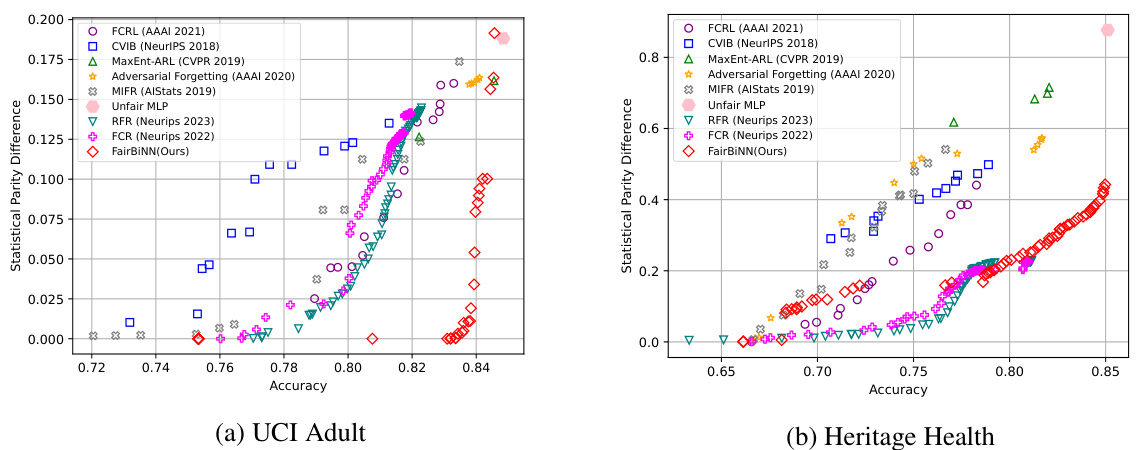
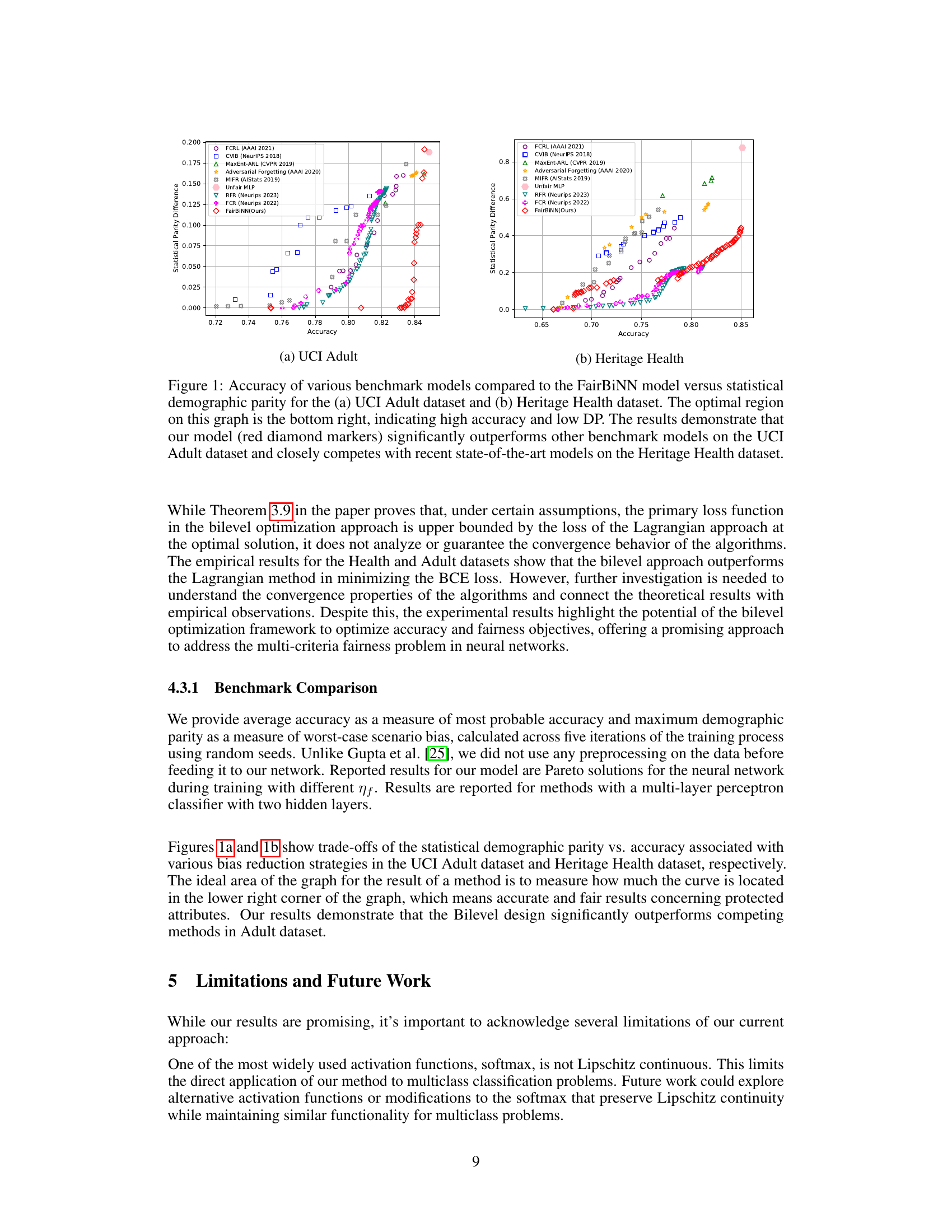
This figure shows the trade-off between accuracy and demographic parity (DP) for different fairness-aware machine learning models on two benchmark datasets (UCI Adult and Heritage Health). The FairBiNN model achieves a better balance between accuracy and fairness compared to the other baselines, demonstrating that the proposed model excels in achieving higher accuracy while maintaining lower DP values, particularly on the UCI Adult dataset.
This table presents the average time taken for one epoch during the training process of two different methods: FairBiNN and the Lagrangian approach. The results are compared for two datasets: Adult and Health. The data shows the computational cost of each method on each dataset. This is useful for evaluating the efficiency of the proposed bilevel optimization method (FairBiNN) relative to the more traditional Lagrangian approach.
In-depth insights#
Fairness Tradeoffs#
Fairness tradeoffs in machine learning represent a core challenge, demanding careful balancing of accuracy and fairness. Algorithmic bias can lead to discriminatory outcomes, impacting vulnerable groups disproportionately. Methods aiming to mitigate bias often involve tradeoffs, where improving fairness might reduce model accuracy, and vice-versa. These tradeoffs are not merely technical; they reflect fundamental ethical considerations and societal values. The choice of fairness metric itself introduces a tradeoff, as different metrics prioritize different aspects of fairness (e.g., demographic parity vs. equal opportunity). Understanding and quantifying these tradeoffs are crucial, requiring not only technical sophistication but also careful consideration of the ethical and societal context. Strategies such as multi-objective optimization or bilevel programming attempt to address this issue by explicitly incorporating fairness as an optimization objective alongside accuracy, providing more control over the resulting fairness-accuracy balance. However, even these advanced methods face limitations and cannot fully eliminate the inherent tension between accuracy and fairness.
Bilevel Optimization#
Bilevel optimization, a powerful technique in mathematical programming, is particularly well-suited for tackling complex problems involving hierarchical relationships. Its core concept revolves around a nested optimization structure, where an upper-level problem optimizes a set of parameters that affect the objective function of a lower-level problem. This hierarchical structure allows for the explicit modeling of interdependencies between objectives. In the context of fairness-aware machine learning, bilevel optimization offers a compelling alternative to traditional Lagrangian methods. The upper level focuses on accuracy, while the lower level aims to improve fairness, thus elegantly balancing the trade-off between these potentially competing objectives. This framework’s effectiveness lies in its ability to capture the nuanced interactions between accuracy and fairness during the training process, leading to superior performance compared to simpler weighted-sum approaches. The theoretical foundation of bilevel optimization, particularly concerning its link to Pareto optimality, provides a robust justification for its use in multi-objective optimization problems.
Empirical Validation#
An Empirical Validation section in a research paper would systematically demonstrate the practical effectiveness of the proposed methodology. It would likely involve applying the method to several real-world datasets, comparing its performance against established baselines, and statistically analyzing the results. Key aspects would include a clear description of the datasets used, their characteristics, and any preprocessing steps. The choice of baselines should be justified, and the evaluation metrics chosen should be relevant to the research question. Robust statistical analysis, including confidence intervals and p-values, is crucial for demonstrating significant improvements. Visualizations, such as graphs and tables, are essential for presenting the results clearly and concisely. A strong Empirical Validation section would build confidence in the claims made in the paper by showing that the proposed approach not only works theoretically, but also delivers tangible benefits in practice. The inclusion of an ablation study, systematically evaluating the impact of individual components of the method, would further strengthen the Empirical Validation and increase the confidence and understanding of its workings.
Theoretical Analysis#
A theoretical analysis section in a research paper would rigorously justify the proposed approach. It would likely begin by formally defining the problem, perhaps as a multi-objective optimization challenge involving accuracy and fairness. Then, the core of the analysis would demonstrate how the method achieves Pareto optimality, ideally showing that improvements in one objective (e.g., fairness) don’t come at the expense of the other (e.g., accuracy). This might involve proving that the method’s solutions satisfy specific conditions for Pareto optimality within a defined solution space. The analysis could also include bounds on the loss function, demonstrating that the proposed method performs at least as well as, or better than, alternative approaches (e.g., Lagrangian methods). Assumptions made during the analysis would need to be clearly stated and their implications discussed. Finally, the analysis should link its theoretical results to the practical application of the proposed approach, highlighting how the theoretical guarantees translate into real-world performance benefits.
Future Directions#
Future research directions stemming from this work could involve exploring the applicability of the FairBiNN framework to a broader range of machine learning models and datasets beyond those considered in this study, such as those involving complex relationships (e.g., graph-structured data) or non-Euclidean spaces. Investigating alternative ways to enforce fairness constraints that may be more robust or less computationally expensive is also warranted. The exploration of different fairness metrics besides demographic parity, along with a deeper analysis of the tradeoffs between accuracy and fairness, would provide a more holistic understanding of the model’s behavior. Finally, more rigorous theoretical analysis and empirical evaluation on larger, more diverse datasets are necessary to solidify the findings and demonstrate the generalizability of FairBiNN. Addressing the inherent challenges of ensuring Lipschitz continuity in complex model architectures and activation functions, such as those commonly used in natural language processing, also presents a significant area for future exploration.
More visual insights#
More on figures
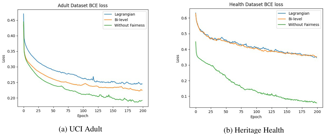
This figure shows the Binary Cross-Entropy (BCE) loss curves for three different training methods (Lagrangian, Bi-level, and Without Fairness) on two datasets (Adult and Health). The Bi-level method consistently achieves a lower BCE loss compared to the Lagrangian method across both datasets, indicating its effectiveness in balancing accuracy and fairness.

This figure shows the accuracy and demographic parity (DP) trade-off for several fairness methods, including the proposed FairBiNN model, on two datasets (UCI Adult and Heritage Health). The results indicate that FairBiNN outperforms the other methods on the UCI Adult dataset and achieves comparable performance on the Heritage Health dataset. The ideal performance is in the bottom right corner (high accuracy, low DP).
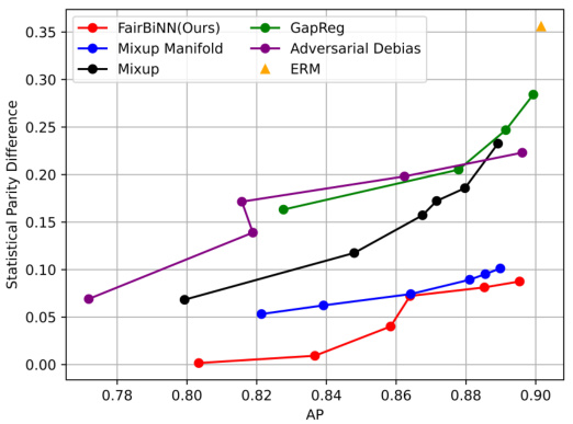
This figure shows the accuracy and demographic parity (DP) of several fairness methods on two datasets: UCI Adult and Heritage Health. The x-axis represents accuracy, and the y-axis represents demographic parity. Lower DP values indicate better fairness. The FairBiNN method (red diamonds) shows superior performance compared to other methods, especially on the UCI Adult dataset. This illustrates the effectiveness of the proposed FairBiNN model in balancing accuracy and fairness.
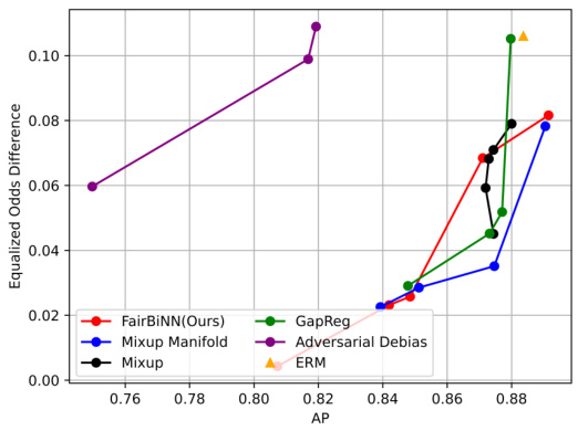
This figure shows the trade-off between accuracy and demographic parity for various fairness-aware machine learning models on two benchmark datasets: UCI Adult and Heritage Health. The x-axis represents the accuracy of the model (higher is better), and the y-axis represents the demographic parity difference (DP), a metric for fairness (lower is better). Each point represents a different model configuration. The ideal location for a point on the graph is the lower right corner (high accuracy and low DP). FairBiNN (the red diamonds) significantly outperforms other models on the UCI Adult dataset and shows competitive performance on the Heritage Health dataset.

This figure shows the trade-off between accuracy and statistical parity difference (SPD, a fairness metric) for the FairBiNN and Lagrangian methods on two datasets: UCI Adult and Heritage Health. Lower SPD values indicate better fairness, and higher accuracy values are preferred. The FairBiNN method consistently achieves better results (closer to the top-left corner, meaning higher accuracy for a given fairness level) than the Lagrangian method. The Heritage Health dataset shows a particularly strong advantage for FairBiNN.

This figure shows a comparison of the FairBiNN model’s performance against other state-of-the-art fairness-aware models. The x-axis represents the accuracy of the model, while the y-axis represents the statistical demographic parity (DP), a measure of fairness. Lower DP values indicate better fairness. The optimal performance is located in the lower-right corner (high accuracy and low DP). The figure demonstrates that FairBiNN significantly outperforms other methods on the UCI Adult dataset and shows competitive performance on the Heritage Health dataset.

This figure presents a comparative analysis of the FairBiNN and Lagrangian methods on two benchmark datasets: UCI Adult (Figure 3a) and Heritage Health (Figure 3b). The graphs plot the trade-off between accuracy and Statistical Parity Difference (SPD), a measure of fairness where lower values indicate better fairness. For the UCI Adult dataset (Figure 3a), we observe that the FairBiNN method consistently outperforms the Lagrangian approach. The FairBiNN curve is closer to the top-left corner, indicating that it achieves higher accuracy for any given level of fairness (SPD). The difference is particularly pronounced at lower SPD values, suggesting that FairBiNN is more effective at maintaining accuracy while enforcing stricter fairness constraints. The Heritage Health dataset results (Figure 3b) show a similar trend, but with a more dramatic difference between the two methods. The FairBiNN curve dominates the Lagrangian curve across the entire range of SPD values. This indicates that FairBiNN achieves substantially higher accuracy for any given fairness level, or equivalently, much better fairness for any given accuracy level. In both datasets, the FairBiNN method demonstrates a smoother, more consistent trade-off between accuracy and fairness. The Lagrangian method, in contrast, shows more erratic behavior, particularly in the Heritage Health dataset where its performance degrades rapidly as fairness constraints tighten.
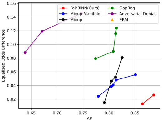
This figure shows a comparison of the FairBiNN model’s performance against several benchmark models on two datasets: UCI Adult and Heritage Health. The x-axis represents the accuracy of the model, while the y-axis represents the statistical demographic parity (DP), a measure of fairness. The ideal region is the bottom right corner, which indicates high accuracy and low DP (high fairness). FairBiNN significantly outperforms the benchmark methods on the UCI Adult dataset and shows competitive performance on the Heritage Health dataset. The plot visualizes the trade-off between accuracy and fairness for each model.

This figure visualizes the results of t-SNE dimensionality reduction applied to the feature embeddings (z and z~) from a ResNet-18 model trained on the CelebA dataset. The left plot (a) shows the embeddings before the fairness layers are added, demonstrating clear separation of gender groups. The right plot (b) shows the embeddings after the fairness layers, demonstrating a lack of separation by gender, indicating successful bias mitigation by the model. The attractive attribute was used for this visualization.

This figure shows the architecture of the FairBiNN model, illustrating how the accuracy and fairness objectives are optimized separately in a bilevel optimization framework. The input layer feeds into the accuracy player’s layers and the fairness player’s layers. The fairness player’s layers aim to minimize the fairness loss function (e.g., demographic parity), while the accuracy player’s layers focus on minimizing the accuracy loss function (e.g., cross-entropy). The outputs of both layers are combined to produce the final classification output.
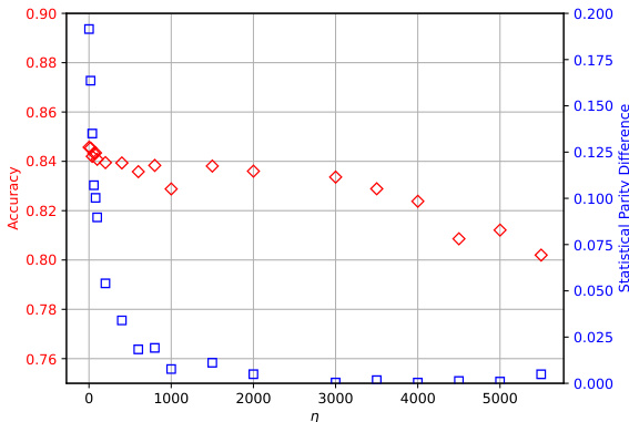
This figure shows the results of an ablation study on the impact of the hyperparameter η on the performance of the FairBiNN model. The study varied the value of η for both Adult and Health datasets, evaluating the model’s performance in terms of accuracy and demographic parity (DP). The results demonstrate that there is a tradeoff between accuracy and fairness as the value of η changes; increasing η leads to improved fairness (lower DP), but at the cost of reduced accuracy. The relationship isn’t linear; diminishing returns are observed in fairness improvements as η increases. The optimal value of η might vary based on the specific needs of applications and the nature of the datasets used.
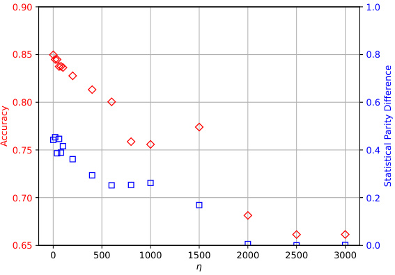
This figure shows the ablation study on the impact of the hyperparameter η on the model’s performance. The hyperparameter η controls the trade-off between accuracy and fairness. The figure contains two subfigures: (a) shows the results on the Adult dataset and (b) shows the results on the Health dataset. Each subfigure shows a scatter plot with the x-axis representing the value of η and the y-axis showing both accuracy (red) and statistical parity difference (blue). As the value of η increases, the statistical parity difference decreases, while accuracy decreases. There is a clear trade-off between accuracy and fairness.

This figure shows the trade-off between accuracy and demographic parity (DP, a measure of fairness) for several fairness-aware machine learning models, including the proposed FairBiNN model, on the UCI Adult and Heritage Health datasets. The x-axis represents accuracy, and the y-axis represents DP. Lower DP values indicate higher fairness. The ideal position for a model is in the bottom right corner (high accuracy, low DP). FairBiNN demonstrates superior performance compared to existing models on the UCI Adult dataset and competitive performance on the Heritage Health dataset.
More on tables

This table presents the average time taken for one epoch during the training process of the FairBiNN and Lagrangian models. The experiments were conducted on an M1 Pro CPU. The results show that the training time for both models is very similar. This empirical finding is consistent with the theoretical computational complexity analysis presented in the paper, where the authors show that both methods have a similar computational complexity.

This table details the hyperparameters used for training the fairness layers in the FairBiNN model on three tabular datasets: UCI Adult, Health Heritage, and a third unnamed dataset. It specifies the number of fully connected (FC) layers before, within (Fairness FC layers), and after the fairness layers; the number of training epochs; batch size; dropout rate; optimizers used for the network and fairness layers; and the learning rates for classifier and fairness layers. Finally, it gives the value of the hyperparameter η, which controls the trade-off between accuracy and fairness in the bilevel optimization framework.
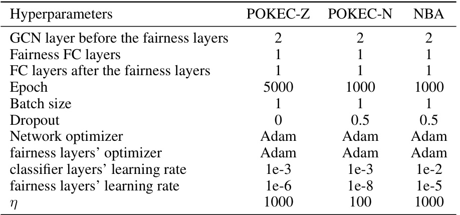
This table lists the hyperparameters used for training the fairness layers on three different graph datasets: POKEC-Z, POKEC-N, and NBA. The hyperparameters include the number of GCN layers before and after the fairness layers, the number of fairness FC layers, the epoch number, batch size, dropout rate, optimizers used for the network and fairness layers, learning rates for both classifier and fairness layers, and the value of eta (η). The differences in hyperparameters reflect the different characteristics and sizes of the datasets.

This table details the hyperparameters used for training the fairness layers in the vision-based experiments using the CelebA dataset. It specifies the number of fairness fully connected (FC) layers, the number of FC layers after the fairness layers, the number of epochs, batch size, dropout rate, optimizers used for the network and fairness layers, and the learning rates for both the classifier and fairness layers. Finally, the η parameter which controls the trade-off between accuracy and fairness is also shown for each of the three different attributes used in the experiments.

This table presents a comparison of the proposed FairBiNN method with various baseline methods on the Pokec-z dataset. The metrics used for comparison are accuracy (ACC), area under the ROC curve (AUC), average demographic parity difference (ADP), and average equalized odds difference (ΔEO). Lower values for ADP and ΔEO indicate better fairness. The results show that FairBiNN achieves comparable or better performance than the baseline methods in terms of both accuracy and fairness.

This table compares the performance of the proposed FairBiNN method against several baseline methods on the Pokec-n dataset. The metrics used are accuracy (ACC), area under the ROC curve (AUC), average demographic parity difference (ADP), and average equalized odds difference (ΔEO). Lower values for ADP and ΔEO indicate better fairness. The results show that FairBiNN achieves comparable or better accuracy than the baselines while also exhibiting significantly better fairness.
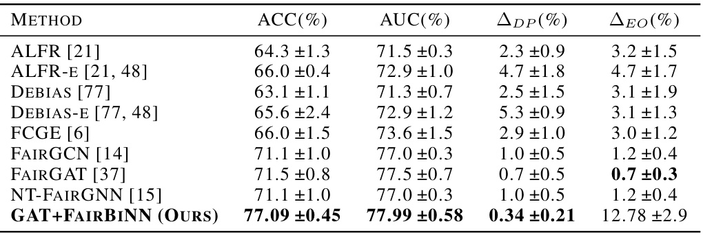
This table compares the performance of the proposed FairBiNN method against several baseline methods for fair classification on the NBA dataset. The metrics used are Accuracy (ACC), Area Under the ROC Curve (AUC), Average Demographic Parity Difference (ADP), and Average Equalized Odds Difference (ΔEO). Lower values for ADP and ΔEO indicate better fairness. The results show that FairBiNN outperforms the baseline methods in terms of accuracy while achieving significantly better fairness.

This table presents the results of an ablation study on the impact of the number of linear layers used in the fairness module of the FairBiNN model. The study compares three configurations: one linear layer, two linear layers, and three linear layers. The Area Under the Curve (AUC) of statistical demographic parity and accuracy are reported for each configuration on the UCI Adult and Heritage Health datasets. The results show a trade-off between fairness and accuracy, with the best performing model varying between datasets.

This table presents a comparison of three different types of fairness layers used in the FairBiNN model: one linear layer, CNN residual block, and a CNN layer. The comparison is based on the average precision (AP), the difference in demographic parity (ΔDP), and the difference in equalized odds (ΔEO) across three different sensitive attributes in the CelebA dataset: attractive, smiling, and wavy hair. The results show that using a single linear layer for the fairness layer resulted in the best performance, specifically in terms of demographic parity and equalized odds. The residual block and the CNN layers are less effective in improving fairness.
Full paper#
